Saturday, April 1, 2017

Strange deep sea creatures

The term deep sea creature refers to organisms that live below the photic zone of the ocean.
These creatures must survive in extremely harsh conditions, such as hundreds of bars of pressure, small amounts of oxygen, very little food, no sunlight, and constant, extreme cold.
Most creatures have to depend on food floating down from above.
These creatures live in very harsh environments, such as the abyssal or hadal zones, which, being thousands of meters below the surface, are almost completely devoid of light.
The water is between 3 and 10 degrees Celsius and has low oxygen levels.
Due to the depth, the pressure is between 20 and 1,000 bars.
Creatures that live hundreds or even thousands of meters deep in the ocean have adapted to the high pressure, lack of light, and other factors.

Friday, March 31, 2017

Reminder : The United States purchased Alaska from the Russian Empire 150 years ago

North western America showing the territory ceded by Russia to the United States
The map the Coast Survey prepared in 1867 still referred to Alaska as “Northwestern America.” 
The Russian settlements are underlined in red.
The Esquimaux settlements are underlined in blue.
With two inset maps: Sitka and its approaches from the Russian and British authorities; and an untitled map showing the North Pacific Ocean including the great circle line from Hakodadi, Japan to San Francisco, California. 
(NOAA/National Archives) Author: United States Coast Survey (1867)
Location: Alaska, Sitka (Alaska)

On this day in 1867, the United States formally took possession of Alaska after purchasing the territory from Russia $7.2 million, or less than two cents per acre.
This purchase increased the nation's size by 586,412 square miles (about two Texas's).

 North America in 1826

The treaty with Russia was brokered by William Seward, the ardently expansionist Secretary of State under President Andrew Johnson.
Many critics believed the land to be barren and worthless, and dubbed the purchase “Seward’s Folly,” "Seward’s Icebox," and “Andrew Johnson’s Polar Bear Garden,” among other ice-cold names.
These critics cooled off following the Klondike Gold Strike in 1896.


Thursday, March 30, 2017

Solving the mystery of the Arctic's green ice

Melt ponds darken the surface of thinning Arctic sea ice, creating conditions friendly to algae blooms under the ice.
(Image courtesy of NASA)

From Harvard by Leah Burrows

In 2011, researchers observed something that should be impossible — a massive bloom of phytoplankton growing under Arctic sea ice in conditions that should have been far too dark for anything requiring photosynthesis to survive.
So, how was this bloom possible?

Using mathematical modeling, researchers from the Harvard John A. Paulson School of Engineering and Applied Sciences (SEAS) found that thinning Arctic sea ice may be responsible for frequent and extensive phytoplankton blooms, potentially causing significant disruption in the Arctic food chain.
The research is described in Science Advances and is a collaboration between researchers from SEAS, University of Oxford and University of Reading.

Arctic Melt Pond
NASA (August 2014)

Phytoplankton underpins the entire Arctic food web.
Every summer, when the sea ice retreats, sunlight hitting the open water triggers a massive bloom of plankton.
These plumes attract fish, which attract larger predators and provides food for indigenous communities living in the Arctic.
Phytoplankton shouldn’t be able to grow under the ice because ice reflects most sunlight light back into space, blocking it from reaching the water below.

Spatial map of the average number of days of sufficient light for sub-ice phytoplankton blooms over time.
(A to C ) Shading indicates the number of days in May,
from 1986 to 1995 (A), 1996 to 2005 (B), and 2006 to 2015 (C), where a sub-ice bloom is permitted. (D to F) Same as (A) to (C) but for June. 

(G to I) Same as (A) to (C) but for July. 
Redboxes in (D) to (F) indicate the region of the 2011 cruise.
Baffin Bay and regions with an ice concentration less than 80% at every point during each time period are colored blue.
Continents are colored gray.


The green shows the area of sea ice where plankton is able to grow (Christopher Horvat)

But over the past decades, Arctic ice has gotten darker and thinner due to warming temperatures, allowing more and more sunlight to penetrate to the water beneath.
Large, dark pools of water on the surface of the ice, known as melt ponds, have increased, lowering the reflectivity of the ice.
The ice that remains frozen is thin and getting thinner.
“Our big question was, how much sunlight gets transmitted through the sea ice, both as a function of thickness, which has been decreasing, and the melt pond percentage, which has been increasing,” said Chris Horvat, first author of the paper and graduate student in applied mathematics at SEAS.
“What we found was that we went from a state where there wasn’t any potential for plankton blooms to massive regions of the Arctic being susceptible to these types of growth.”

Scientists have made a biological discovery in Arctic Ocean waters as dramatic and unexpected as finding a rainforest in the middle of a desert.
A NASA-sponsored expedition punched through three-foot thick sea ice to find waters richer in microscopic marine plants, essential to all sea life, than any other ocean region on Earth.
The discovery is the result of an oceanographic expedition called ICESCAPE, or Impacts of Climate on EcoSystems and Chemistry of the Arctic Pacific Environment.
The NASA-sponsored mission explored the seas along Alaska's western and northern coasts onboard a U.S. Coast Guard icebreaker during the summers of 2010 and 2011.
The finding reveals a new consequence of the Arctic's warming climate and provides an important clue to understanding the impacts of a changing climate and environment on the Arctic Ocean and its ecology. 

The team’s mathematical modeling found that while the melt ponds contribute to conditions friendly to blooms, the biggest culprit is ice thickness.
Twenty years ago, only about 3 to 4 percent of Arctic sea ice was thin enough to allow large colonies of plankton to bloom underneath.
Today, the researchers found that nearly 30 percent of the ice-covered Arctic Ocean permits sub-ice blooms in summer months.
“The meter decline in sea ice thickness in the Arctic in the past 30 years has dramatically changed the ecology in that area,” said Horvat.
“All of a sudden, our entire idea about how this ecosystem works is different. The foundation of the Arctic food web is now growing at a different time and in places that are less accessible to animals that need oxygen.”

Links :

Wednesday, March 29, 2017

Scientists trace South Georgia's giant ice history

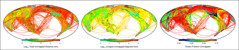
Overview of sea-floor landforms mapped in this study

From BBC by Jonathan Amos

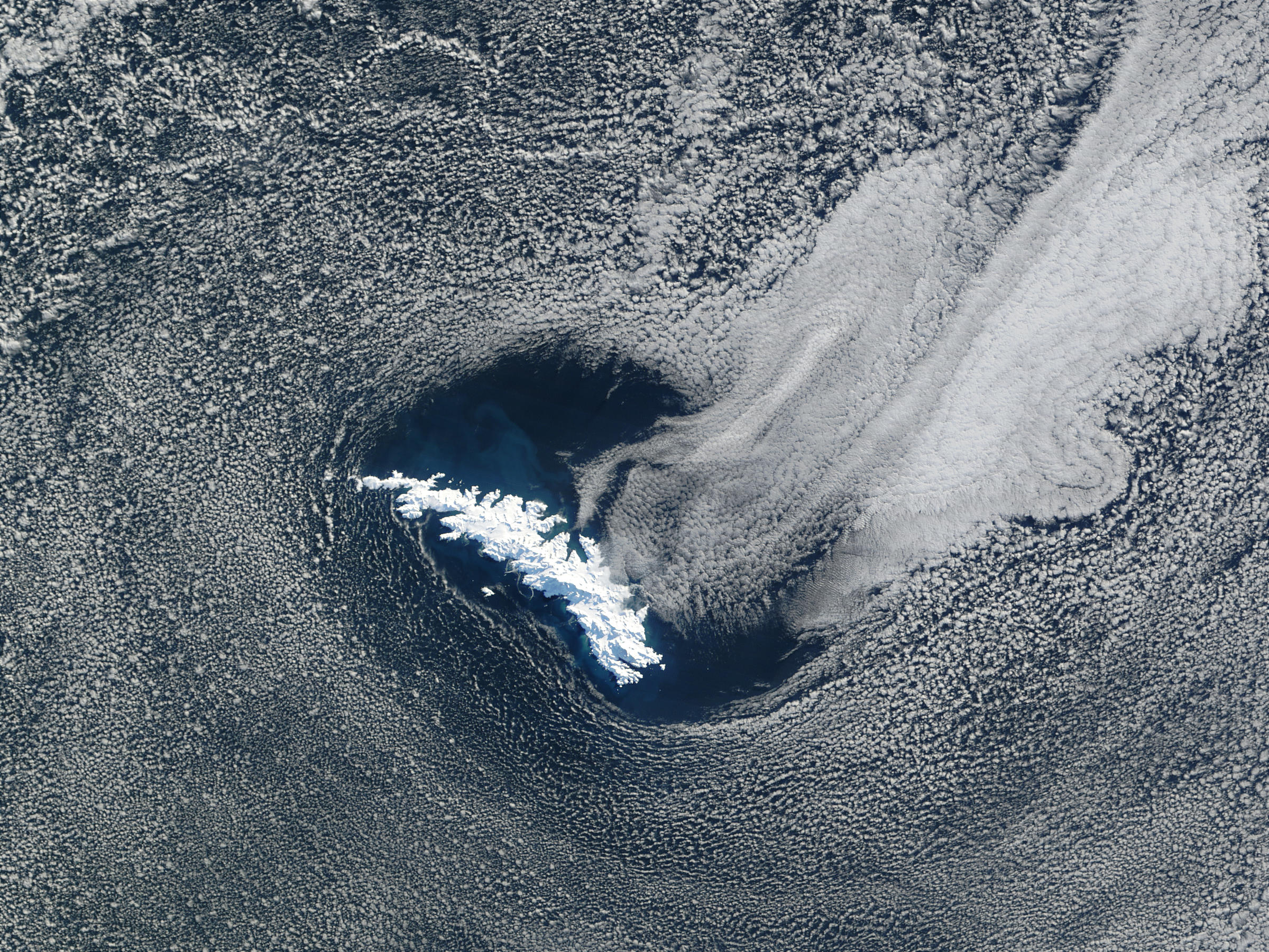
South Georgia is an island of astonishing beauty - of imposing landscapes, and bewildering numbers of penguins, seals and seabirds.
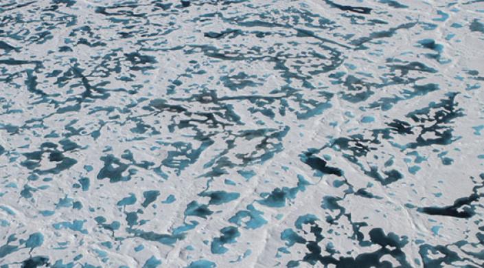
It also has some impressive ice fields, although none it seems quite like those of the past.
Some 20,000 years ago the island's glaciers pushed out 50km and more from their current positions, reaching to the edge of the continental shelf.
The British Overseas Territory was in effect covered by a giant ice cap.
This realisation is reported in the current edition of the journal Nature Communications.

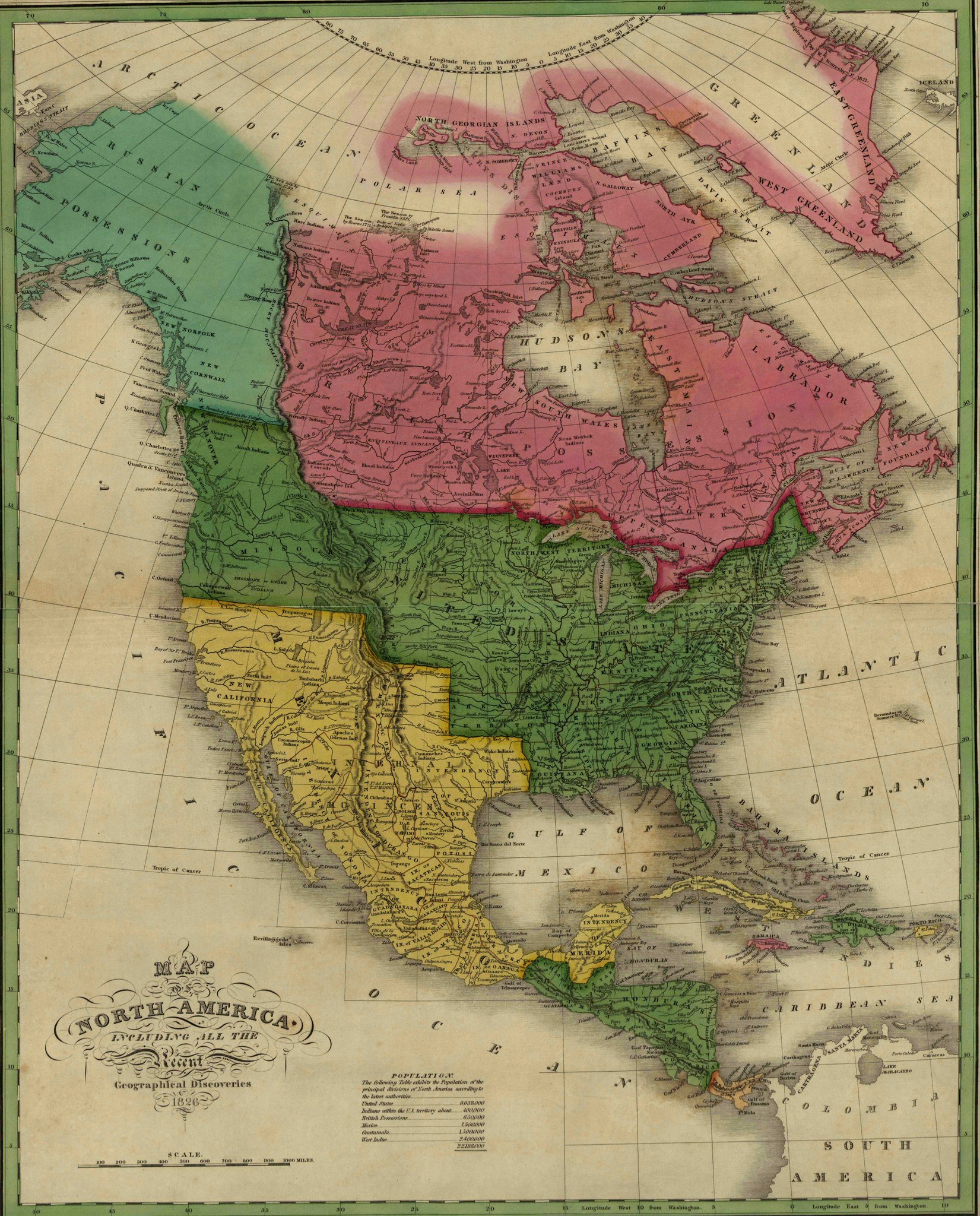
 South Georgia (UKHO map) in the GeoGarage platform
Located in the Southern Atlantic Ocean roughly 1,700 miles (2,735 km) due east of Argentina’s southernmost tip, South Georgia Island was a stop-over point for Sir Ernest Shackleton in November 1914. 

It is the result of investigations of the seafloor by a team of scientists from the UK, Germany and Australia.
"We were able to find a tracer of this ice cap - a ridge at the outer margin of the continental shelf that's larger than all others, pretty much; and it's fairly contiguous," explained Dr Alastair Graham from Exeter University.
"You see it to the west, to the north, to the east, and even to the south where we don't have much data. It's quite a surprise because many scientists had assumed any ice cap was quite small."
Dr Graham and his colleagues conducted sonar surveys around South Georgia using the British Antarctic Survey's (BAS) research vessel, the James Clark Ross, and Germany's RV, the Polarstern.

 Map of South Georgia
(a) Southern Hemisphere map showing sites where advances of glaciers during the Antarctic Cold Reversal have been recorded.
(b) Regional location map illustrating modern-day mean annual position of major Southern Ocean oceanographic fronts in relation to South Georgia.

These ships mapped the long deep troughs cut by ancient glaciers.
Evident in these channels are the countless, tell-tale markings of bulldozed sediments known as moraines.
But to fill out their picture, the researchers needed also to establish when these features were produced, and so they pulled up cores of seafloor material.
Caught up in this mud and rock are the shelly remains of tiny animals that can be used to date the glacial deposits.
What emerges from all this study is a story of a rapidly changing ice-scape - one that has been incredibly sensitive to really quite small changes in temperature.

The investigation reveals that the giant ice cap was at its fullest extent at the height of the last ice age - about 19 to 26 thousand years ago.
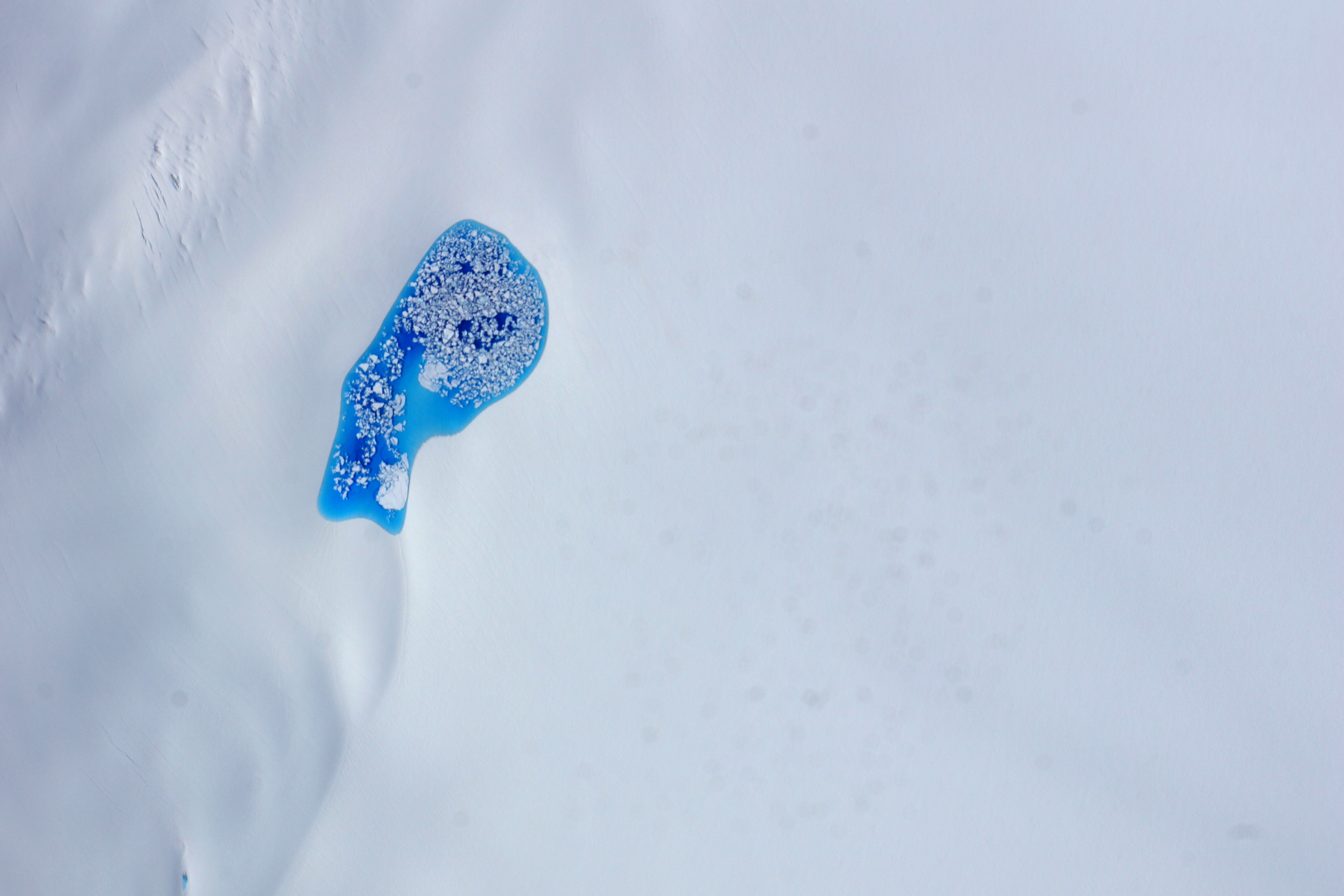
Then, as the global climate warmed, the glaciers went into a fast retreat, pulling back to positions not far beyond the present coastline.
A pulse of cooling about 15,000 years ago saw them briefly push forward, before deglaciation took hold again.
"In the last 10,000 years the ice cap has wobbled back and forth, but never really gone out much beyond the fjords," Dr Graham told BBC News.
"And then in the 1950s, things seemed to go pear-shaped for South Georgia. The glaciers now are in a massive retreat, which could have quite serious implications for local ecosystems."

 (a) Location map indicating the locations of panels bg.
(b) Streamlined crag-and-tails and/or drumlins 0.5–1 km in length, south of Undine South Harbour;
(c) streamlined bedforms and roche moutonnée overprinted by extensive scouring in the trough feeding out of Drygalski Fjord;
(d) elongated mega-scale glacial lineations and
(e) drumlinoid bedforms that increase in elongation down-flow in the trough northwest of Church Bay;
(f) convergence of flow patterns including a swarm of small drumlins at the confluence of tributaries emanating from Possession Bay and Antarctic Bay;
(g) individual drumlin imaged on flat sea-bed region south of the central part of the island.
All multibeam data have an 8 m grid-cell size, except for ‘f’ which is gridded at 20-m cell size. Arrows depict direction of former ice flow.

 The Cumberland Trough - the seafloor scar left by a once mighty glacier
  • General context map (1) for Cumberland Bay in central-north South Georgia
  • Bathymetry reveals a large trough (2) spreading northeast for up to 70km
  • Numerous ridges (2) of bulldozed sediment (moraines) cross the trough
  • (3) Downstream of today's Nordenskjold Glacier is one large moraine
  • This ridge (3) is probably the extent of a brief re-advance 15,000 years ago
(a) Compiled swath bathymetry tracks west of the island illustrating a large outer ridge and back-stepping recessional moraines; profile v–x through the ridge shown in ‘c’; 
(b) a sub-set of the recessional moraines in detail.
(c) profile v–x through the outer ridge showing the separation of deeper, pitted sea-floor and moraine-mantled topography inshore.
(d) streamlined subglacial bedforms south of the island, resembling drumlins formed by warm-based, fast glacial flow. 
(e) topographic profile y–z across the bedforms illustrating their range of amplitudes and typical wavelengths. Profile located in ‘d’. Data in ‘a’ gridded at 5 m grid cell size, and at 8 m grid-cell size in ‘d’.

With so many of the glaciers today pulling back on to land, they no long provide as much crushed rock to the surrounding ocean as they once did.
This potentially could put new constraints on the bio-productivity of the region, said co-worker Prof Dominic Hodgson from BAS.
"As they erode, South Georgia and the other sub-antarctic islands put 'rock flour' in the ocean and that provides a supply of iron. Iron is the limiting nutrient," he explained.
"It gives rise to big blooms of plankton which then drive the ecosystem from the bottom up - from the plankton and zooplankton, to the krill, all the way up to the seals, birds and penguins. This is why you get this intense concentration of biota around South Georgia."

South Georgia Island
NASA (2002) 

Eastern half of South Georgia Island
Today, the glaciers are in an accelerated reversal, with many pulling back up on to the land 
(ISS NASA 2013)

It is an interesting question, however, as to what all this wildlife did when South Georgia was covered by a huge ice cap.
Many of its bird species, such as the albatrosses for example, nest in burrows and so need some clear, ice-free land to breed.
There are also some endemic animals - they exist nowhere else.
For these creatures to have survived through the great glaciation there must have been gaps in the ice cap.
The team is trying to establish where these refugia might have been.
Another spillover from the study is determining what the South Georgia experience tells us about higher latitudes, such as the Antarctic Peninsula.

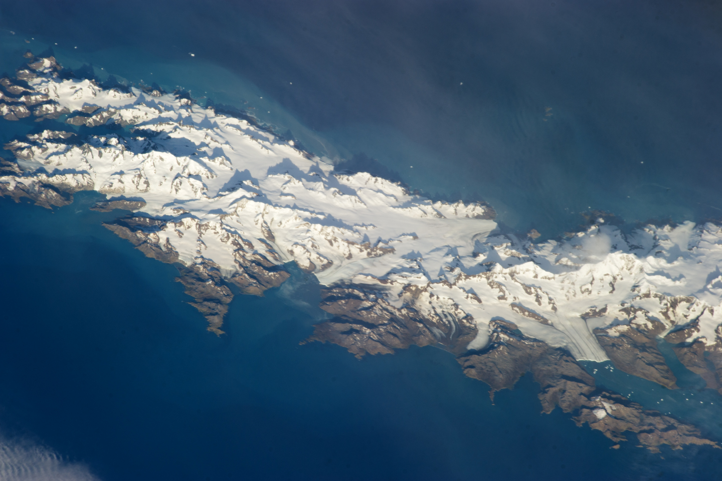
 Away from the brutal westerlies, South Georgia has some green spaces

The glaciated "finger" of land that juts up from the White Continent towards South America is already one of the fastest warming locations on Earth.
Scientists who try to model its future behaviour now have a new anchor point in their simulations thanks to this study.
"South Georgia shows us what the response is of an ice sheet to really very moderate changes in temperature, both in the ocean and the atmosphere," said Prof Hodgson.
"We can now take those responses and push them further south and get a very good idea of what might happen to the Antarctic Peninsula, and indeed any ice sheet that is close to its thermal limit."

Links :

Tuesday, March 28, 2017

Airline flight paths over the unmapped ocean

Depth measurements available at the time of flights MS804, MH370 and AF447 crashes

From EOS by , Karen M. Marks, and Thierry Schmitt

An assessment of ocean depth knowledge underneath commercial airline routes shows just how much of the seafloor remains "terra incognita."

It has been 3 years since Malaysia Airlines flight MH370 disappeared, and no trace of it on the seafloor has yet been found. MH370 is believed to have deviated from its intended flight path.
Yet even the typical routes taken by overseas flights are often over unknown seafloor.

In fact, of the total over-ocean distance covered by all unique overseas flight routes, 60% is above unmapped areas.
The quality of mapping that does exist varies widely, and the lack of data and variance in quality hinder searches for missing aircraft, hazard assessments, and the pursuit of baseline scientific knowledge.
A modest effort could fix this lack of data.

Shaded relief images of 800*600km regions in search areas of MS804, MH370 and AF447.

Uneven Coverage

Only a small percentage of Earth’s seafloor has been mapped [Copley, 2014; U.S. National Ocean Service, 2014].
For example, Smith and Marks [2014] reported that only 5% of the southeast Indian Ocean seafloor was covered by echo soundings on 8 March 2014 when Malaysia Airlines flight MH370 went missing.
Since their publication, the MH370 search area was moved to an area where data coverage was only 1% at the time the aircraft was lost.
In January 2017, the search was suspended after 120,000 square kilometers had been mapped in efforts to find the aircraft.
This is roughly 1/3 of the area shown in Figure 1 and 0.0336% of the area of Earth’s ocean floor.

Bathymetry of Mediterranean sea (GEBCO)

In contrast, 86% of the eastern Mediterranean seafloor is mapped in the region where EgyptAir flight MS804 crashed on 19 May 2016, and 30% of the equatorial Atlantic is mapped where Air France flight AF447 fell on 1 June 2009.
Comparing these three search regions at the same scale shows that ocean mapping varies enormously from region to region (Figure 2).
The AF447 search region also illustrates the strong bias toward mapping of mid-ocean ridges at the expense of other areas [Smith, 1998].

Following the Airplanes

To illustrate the extent of ocean mapping under aviation routes, we compiled a list of these routes using data from the Open Flights project on GitHub.
These data list the originating and terminating airports of regularly scheduled commercial flights and whether or not the service is nonstop.
The actual path taken by any particular flight is determined as air traffic controllers direct each flight to a sequence of waypoints and may change as weather and traffic loads change.
We did not have this level of detail, so we approximated flight routes as great circles connecting the originating and terminating airports.
Since the Open Flights data do not indicate the locations of intermediate stops, we analyzed only nonstop routes.
Some pairs of airports (e.g., New York’s Kennedy and London’s Heathrow) are served by many airlines flying many flights in each direction, but our analysis used each unique pair of airports only once, regardless of the frequency of flights between its airports.
We generated a great circle route connecting each airport pair, sampled that route every 1 kilometer of distance along its path, and then classified each sample point as being over mapped ocean, over unmapped ocean, or not over ocean.

left: total distance over unmapped ocean,
middle: longest segment of any route over unmapped ocean,
right: relative fraction of each route that over unmapped ocean

We found that the total distance along any individual route includes as many as 9201 kilometers flown over unmapped ocean (Figure 3, left).
Half of all over-ocean routes fly more than 200 kilometers over unmapped ocean, and 10% of the over-ocean routes fly more than 2000 kilometers over unmapped ocean.
The longest contiguous unmapped ocean segment along any one route (Figure 3, middle) is 2293 kilometers, traveled when flying between New York’s John F. Kennedy and Beijing’s Chongqing airports, and more than 20% of routes have a longest unmapped segment exceeding 200 kilometers. On most routes, more than half of the over-ocean portion is over unmapped ocean (Figure 3, right).

We found a total of 19,024 unique nonstop routes.
Of these, 11,665 fly at least 1 kilometer over ocean, and 10,686 fly at least 1 kilometer over unmapped ocean. The total route distance is slightly more than 33.4 million kilometers, 33% of which is over ocean, with 60% of the total over-ocean distance being over unmapped ocean.
These numbers do not indicate the probability that an aircraft or a passenger is over unmapped ocean because our analysis is unable to account for the number of aircraft and passengers flying each route over a given period of time.

Our Criteria

An analysis like our airline route survey has to define how many depth readings it takes to list an area as mapped.
Depth measurements that can be readily obtained and used without specialized access, licensing, or payment, which we call “available” data, are quite variable in their sampling density and in the age, technology, and accuracy of the sounding and navigation systems used.
All these variations are irregularly distributed over the globe [Smith, 1993; Wessel and Chandler, 2011].
We divided the global seafloor area into equal-area square tiles 1 nautical mile on a side and considered any tile mapped if it contained one or more available echo soundings.
For context, modern hull-mounted multibeam echo sounders (MBES) map a swath of the ocean along the ship’s path, but the vast majority of available data (95% of coverage by area) are point values—one depth measurement at one place, typically an analog measurement made by a wireline or a single-wide-beam acoustic sounder [Smith, 1993].

Our method produces a generous overestimate, with some tiles having only one sounding.
Also, the majority of available data are poorly navigated and error prone [Smith, 1993; Wessel and Chandler, 2011].
Even by this generous definition, however, only 8% of the global ocean is mapped [Wessel and Chandler, 2011, Figure 8].
In the 92% of ocean area where depth has not been measured, satellite altimetry interpolates the gaps between available soundings [Smith and Sandwell, 1997; Becker et al., 2009; Weatherall et al., 2015]. This approximation strongly underestimates seafloor topography and roughness [Becker and Sandwell, 2008], with a variety of consequences that affect sciences, from earthquake and tsunami hazard assessment [Mofjeld et al., 2004] to ocean circulation [Gille et al., 2004] and mixing [Kunze and Llewellyn Smith, 2004] and climate forecasts [Jayne et al., 2004].

 BA4000 : the UKHO World map in the GeoGarage nautical charts platform

Addressing the Data Shortage

All of Earth’s ocean floors deeper than 500 meters could be mapped at a total cost of $2–3 billion.
All of Earth’s ocean floors deeper than 500 meters (i.e., exclusive of territorial waters and continental shelves) could be mapped by GPS-navigated MBES for 200 ship-years of effort (e.g., 40 ships working for 5 years), at a total cost of US$2–3 billion [Carron et al., 2001].
According to the NASA scientists we consulted, this is less than the cost of NASA’s next mission to Europa.
We hope that our survey of the state of ocean mapping from the perspective of over-ocean flight routes makes the relevance of ocean mapping and the current lack of mapping information clear to the public.

Links :

Monday, March 27, 2017

New International Cloud Atlas: 19th century tradition, 21st century technology


From WMO

The World Meteorological Organization (WMO) has released its new, long-awaited, digitized International Cloud Atlas – the global reference for observing and identifying clouds, which are an essential part of weather, the climate system and the water cycle. It was released for the World Meteorological Day on 23rd March.

The new Atlas combines 19th century traditions with 21st century technology.
It contains hundreds of images submitted by meteorologists, photographers and cloud lovers from around the globe.
It includes new classifications, including volutus, a roll cloud; clouds from human activities such as the contrail, a vapour trail sometimes produced by airplanes; and asperitas, a dramatic undulated cloud which captured the public imagination.
It also features meteorological phenomena like rainbows, halos, snow devils and hailstones.

NOAA

“The International Cloud Atlas is the single most authoritative and comprehensive reference for identifying clouds. Its reputation is legendary among cloud enthusiasts and it serves as an essential training tool for professionals working in meteorological services, and in sectors such as aviation and shipping,” said WMO Secretary-General Petteri Taalas.
“Throughout the centuries, few natural phenomena have inspired as much scientific thought and artistic reflection as clouds,” said Mr Taalas.
“More than two millennia ago, Aristotle studied clouds and wrote a treatise addressing their role in the hydrological cycle. And today, scientists understand that clouds play a vital role in the Earth’s energy balance, climate and weather,” said Mr Taalas in a message for World Meteorological Day on 23 March.
“If we want to forecast weather we have to understand clouds. If we want to model the climate system we have to understand clouds. And if we want to predict the availability of water resources, we have to understand clouds,” said Mr Taalas.


Understanding Clouds is the theme of this year’s World Meteorological Day, which celebrates the anniversary of the convention establishing WMO in 1950 and showcases the essential contribution of National Meteorological and Hydrological Services to the safety and wellbeing of society.
The themes chosen for World Meteorological Day reflect topical weather, climate or water-related issues.
Understanding Clouds was chosen to coincide with the launch of the digital version of the International Cloud Atlas, after an exhaustive revision process and a public call for images from all over the world.

courtesy of the Cloud Appreciation Society (2009)

19th Century Traditions

The International Cloud Atlas was first published in the late 19th century.
It contains a detailed manual of standards and numerous plates of photographs of clouds and certain other weather phenomena.
It was last updated in 1987 – before the Internet era.
For the first time, the 2017 edition will primarily be a web-based portal, allowing for much richer content and presentation. It may be published in hard copy at a later date.
“This is THE world reference for observing and classifying clouds and other weather phenomena. The Atlas contains pictures, definitions, and explanations that are accepted and used by all WMO’s 191 Member countries and territories,” said Bertrand Calpini, President of WMO’s Commission for Instruments and Methods of Observation (CIMO), which oversaw the revision process.
“This new edition brings together for the first time all types of measurements, including  very high-tech surface-based, in situ and space observations and remote sensing, thus giving to the human observer a revolutionary tool to understand clouds,” said Mr Calpini.
“The International Cloud Atlas task team had to choose from thousands of images from meteorologists, cloud lovers and photographers around the world,” said Chi-ming Shun, Director of the Hong Kong Observatory, which is hosting the web portal.
“We selected the best of the best.  We feel honoured to be involved in such a visible product of WMO. We applaud WMO for updating the International Cloud Atlas which provides a unique platform for engaging the public in better understanding clouds, weather and climate.”

The new classifications are available here

Classification of Clouds
The present international system of Latin-based cloud classification dates back to 1803, when amateur meteorologist Luke Howard wrote The Essay on the Modifications of Clouds.
There are ten basic cloud “genera,” which are defined according to where in the sky they form and their approximate appearance.
The new International Cloud Atlas has made no additions to these 10 genera.
High-level clouds typically have a base above about 5 000 metres (16 500 feet); middle-level clouds have a base that is usually between 2 000 and 7 000 m (6 500 to 23 000 feet); and low-level clouds usually have their base at a maximum of 2 000 m (6 500 feet).
Most cloud names contain Latin prefixes and suffixes which, when combined, give an indication of the cloud’s character. These include:
  • Alto: mid-level (though Latin for high)
  • Cirrus/cirro: feathers, wispy
  • Cumulus/cumulo: heaped up/puffy
  • Nimbus/nimbo: rain-bearing
  • Stratus/strato: flat/layered and smooth
The 10 genera are subdivided into “species,” which describe shape and internal structure, and “varieties,” which describe the transparency and arrangement of the clouds. In total there are about 100 combinations.

Altocumulus volutus

The new International Cloud Atlas has added a new species: volutus or roll cloud (from the Latin volutus which means rolled), which occurs within the genera Altocumulus and Stratocumulus.
It describes a long, typically low, horizontal tube shaped cloud mass that often appeals to roll about a horizontal axis.
Five new supplementary features have been added: asperitas, cavum, cauda (often known as tail cloud), fluctus (widely known as Kelvin-Helmholz wave) and murus (known as wall cloud).
Best known of these is asperitas (from the Latin meaning roughness), Photographs of the dramatic, wave-like cloud captured the popular imagination around the world.
The Cloud Appreciation Society argued for a new classification to be used to describe clouds with this appearance.

 The wavy ridges of the rare asperitas cloud

The Atlas includes the winning photograph from a Cloud Appreciations Society competition on Asperitas.
“Asperitas was first identified with the help of citizen science, enabled by modern technology. When Cloud Appreciation Society members send us photographs of dramatic skies from around the world, it is possible to spot patterns. This is how the proposal for a new classification came about, and we are delighted the WMO has chosen to include it in their definitive reference work for cloud classification,” said Gavin Pretor-Pinney, founder of the Cloud Appreciation Society.

A new accessory cloud, flumen, has been included. Commonly known as “beaver’s tail,” it is associated with a supercell severe convective storm.
The International Cloud Atlas also proposes five new “special clouds:” cataractagenitus, flammagenitus, homogenitus, silvagenitus and homomutatus.
The suffix genitus indicates localized factors that led to cloud formation or growth, while mutatus is added when these caused the cloud to change from a different form.
These special clouds are influenced by large waterfalls, localized heat from wildfires, saturation of air above forests and humans.
Thus, a common example of homogenitus is contrails, sometimes seen after aircraft.
The World Meteorological Day ceremony will be webcast live to allow cloud enthusiasts around the world to have their first view of the new International Cloud Atlas and the new insight it provides into the beauty and power of nature.

Links :

Sunday, March 26, 2017

Copulating seahorses and a lavish snail ballet: the underwater wonders of Jean Painlevé


From The Guardian by Hettie Judah

They may have infuriated the censor, but these beautiful films and photographs of cavorting creatures caused a sensation in the 30s.
As Ikon’s new exhibition shows, they have been overlooked for too long

 Desperately seeking the nose of a shrimp …
Jean Painlevé with his camera in a waterproof box, 1935
Photograph: Image courtesy of Archives Jean Painlevé, Paris

In the course of his lifetime, the aquatic French film-maker Jean Painlevé hung out with Man Ray and Alexander Calder, showed his work in galleries alongside the surrealists, and inspired George Balanchine to choreograph a lobster ballet.
His most successful film, 1934’s L’Hippocampe ou Cheval Marin, didn’t just incur the wrath of censors with its intimate footage of copulating seahorses.
It also provoked such a mania for the arresting little creatures that the Frenchman, somewhat improbably, launched a range of fashion accessories.
Overlooked for decades, PainlevĂ©’s curious – and curiously beautiful – underwater movies have been championed by France’s current crop of global art stars, among them Pierre Huyghe and Philippe Parreno.
In recent years, his aquatic films have been seen in group exhibitions, becoming a point of reference for the art world’s mounting obsession with the animal kingdom.
Now Ikon in Birmingham is presenting his first British solo show.

A still from The Seahorse, 1931.
Photograph: Courtesy of Archives Jean Painleve, Paris 

It’s not often an exhibition is given its own bespoke wallpaper but, in keeping with the joy and playfulness of PainlevĂ©’s underwater explorations, this show is something of a peculiarity itself.
The wallpaper, which enlivens the opening gallery, is a coral and seahorse design created by PainlevĂ©’s partner Geneviève Hamon for a silk scarf.

The exhibition captures the range of PainlevĂ©’s output in a career that stretched from the 1920s to the 70s.
On the walls hang intimate shots – the nose of a shrimp, the horn of a seahorse, the suckers of an octopus – all made with a microscope.
Taken in the 1920s and 30s, when Painlevé exhibited them blown up to monstrous dimensions, they are crisp, luminous and mysterious.


Of the four films shown, two are studies of aquatic creatures: the famous seahorses and the tiny Acera sea snails.
Both are oddly erotic in places. Painlevé allowed himself to be transported by his own delight in unexpected phenomena.
In the case of the Acera, these include hermaphroditic mating practices and a lavish, highly balletic dance, in which the snails use their tiny shells as ballast while they shoot themselves up and down in the water.
PainlevĂ© sets this against music by Pierre Jansen – a composer best known for his work with Claude Chabrol – with each swoop echoed in the music, as though they were performing to a score for waltzing lovers.

Surreal sea … Crab Claw, 1928.
Photograph: Courtesy of Archives Jean Painlevé, Paris

While this may sound like something straight out of The Life Aquatic With Steve Zissou, PainlevĂ©’s methods were rather more homespun than those of Wes Anderson’s titular hero.
In place of leopard sharks tracked in a minisub, the stars of PainlevĂ©’s movies were tiny creatures – shrimp, squid, octopus, slug – caught by hand in shallow waters off the coast of Brittany.
Most of PainlevĂ©’s films were made in aquariums in his studio laboratory, some double-walled to protect the inhabitants from the heat of the lights.
Beside the film-maker’s enthusiasm for his tiny subjects, what stands out is the use of cutting-edge and scientific equipment – underwater cameras and microscopy – that offered a new glimpse of this little-known world.
Of the other two films, one – a distinctly psychedelic study of the proliferation of liquid crystals – underscores PainlevĂ©’s status as a scientist.
The other, which shows Alexander Calder operating a mechanical circus created in the 1920s, is a reminder of the film-maker’s close ties to the art world. Membership of the French Union of Communist Students in his younger days had also put PainlevĂ© in touch with avant-garde film-makers including Luis Buñuel and Sergei Eisenstein, and he went on to speak and write extensively about his creative philosophies.


In 1948, he suggested Ten commandments of film-making, warning against the over-reliance on special effects and the use of monotonous sequences.
For all his associations with the avant-garde, PainlevĂ©’s great ambition was that his films would reach the widest possible audience, spreading his enthusiasm and scientific knowledge.
They are, to this end, unapologetically entertaining, often highly anthropomorphic.
Watching the male seahorse eject hundreds of tiny babies from its pouch, Painlevé notes what seems to be alarm in the darting of its eyes, likening the whole experience to the contractions of human labour.
Part of L’hippocampe’s sensational success can be attributed to how its subjects upturned gender roles, something PainlevĂ© clearly approved off, since one of his Commandments decrees: “You will refuse to direct a film if your convictions are not expressed.”
Narrating to some footage of female seahorses impregnating the male with eggs, Painlevé was emphatic in his approval, and no less enthusiastic about the subsequent division of labour in pregnancy and parenthood.
There’s some aquatic-themed costume jewellery on show in a glass vitrine here.
To the casual eye, it may seem a little out of place, but don’t be fooled.
That sea horse motif was a potent symbol of equality.

Links :