Saturday, December 23, 2023

Panama canal ancient maps

Maps of proposed Panama Canal between Gorgona and Panama City]. Section A (1895 ?)
source : LOC 
 

1895 Compagnie Nouvelle du Canal de Panama Map of the Panama Canal

1911 Antique PANAMA CANAL Map of the Panama Canal
 
Panama Canal - Pacific Coast Approaches - 1913
 
1916 
 
 1921

Friday, December 22, 2023

The extended continental shelf (ECS) : announcement of U.S. Extended Continental Shelf Outer Limits

The World Map of Extended Continental Shelf Areas depicts areas of ECS asserted by coastal States worldwide, as of the date of publication of this map.
Combined, these ECS areas cover approximately 9% of the ocean’s seabed.

 
Unilateral declaration of extension of the continentalshelf by the United States.
Note : The United States have not ratified the United Nations Convention on the Law of the Sea (UNCLOS). They therefore cannot have their claims validated by the Commission on the Limits of the Continental Shelf (CLCS)
 
The continental shelf

The continental shelf is the extension of a coastal State’s land territory under the sea. Under customary international law, as reflected in Article 76 of the 1982 Law of the Sea Convention (Convention), the continental shelf consists of the seabed and subsoil that extends (1) to the outer edge of the continental margin, or (2) to a distance of 200 nautical miles from the coast if the outer edge of the continental margin does not extend up to that distance.
This legal definition is different from the geological definition of a continental shelf.
The continental shelf is an important maritime zone that holds many resources and vital habitats for marine life.

The extended continental shelf (ECS)

The extended continental shelf, or ECS, refers to that portion of the continental shelf beyond 200 nautical miles from the coast (Figure 1).
See the World Map of ECS areas above.
ECS is a term of convenience; under the Convention, the term “continental shelf” includes both continental shelf within and beyond 200 nautical miles.

Figure 1: Maritime zones under the international law of the sea. ECS is that portion of the continental shelf that extends beyond 200 nautical miles.
 
Determining the outer limits of the ECS

Determining the outer limits of the ECS is different from determining the extent of other maritime zones, such as the territorial sea and exclusive economic zone. 
 These other maritime zone limits are determined based on a specified distance from the coastal baselines (Figure 1).

The outer limits of the ECS, however, depend on the geophysical characteristics of the seabed and subsoil. ECS limits are determined using complex provisions set forth under Article 76 of the Convention. (The text of Article 76 can be found here. )
A coastal State can use one of two formulas in any combination to determine the outer edge of its continental margin (Figure 2).
Article 76 also contains two constraint lines (Figure 3).
If the outer edge of the continental margin extends past the constraint lines, a coastal State can use either of the constraint lines to maximize its ECS.
The outer limit of the continental shelf is determined by the combined use of Article 76’s formula lines and constraint lines.

As discussed in the Data Collection section of the U.S. ECS website, bathymetric and seismic data are needed to apply the formula and constraint lines.
 
Figure 2: Formula lines under Article 76 of the Law of the Sea Convention. A coastal State can use either formula to determine the outer edge of the continental margin.
 
Figure 3: Constraints under Article 76 of the Law of the Sea Convention.
A coastal State can use either constraint to maximize the limits of its continental shelf.
 
Continental shelf rights

The sovereign rights and jurisdiction of a coastal State over its continental shelf are reflected in the Convention and include the following:Conservation, management, and use of living and non-living resources
Regulating marine scientific research
Construction, operation, and use of artificial islands, installations, and structures
Delineating the course for laying pipelines
Drilling for any purpose
Prevention of marine pollution in connection with some activities
 
Distinction between the continental shelf and EEZ

The continental shelf and the exclusive economic zone (EEZ) are distinct maritime zones (Figure 1). The continental shelf includes only the seabed and subsoil, whereas the EEZ also includes the water column.
In addition, while the maximum extent of the EEZ is 200 nautical miles from the coast, the continental shelf may extend beyond 200 nautical miles, depending on the depth, shape, and geophysical characteristics of the seabed and sub-sea floor.
The ECS is, therefore, not an extension of the EEZ. Some of the rights that a coastal State may exercise in the EEZ, especially rights over water column resources (e.g., fish), do not apply to the ECS. 
 
The United States has ECS in seven offshore areas (Figure 1): the Arctic, Atlantic (east coast), Bering Sea, Pacific (west coast), Mariana Islands, and two areas in the Gulf of Mexico.
The U.S. ECS area is approximately one million square kilometers – an area about twice the size of California.
The United States may also have ECS in other areas, and the U.S. ECS Project continues to analyze available data and undertake analysis in a range of areas. 
 
What is the ECS?
The continental shelf is the extension of a country’s land territory under the sea.
The continental shelf holds many resources (e.g., corals, crabs) and vital habitats for marine life.
The portion of the continental shelf beyond 200 nautical miles from the coast is known as the “extended continental shelf,” or ECS. The ECS includes the seabed and subsoil, but not the water column.
 
The Arctic Region of the U.S. continental shelf is located in the Arctic Ocean, north of the U.S. state of Alaska.
This region is bounded by Canada to the east and the Russian Federation to the west.
The extended continental shelf of the United States in this region extends north to a distance of 350 nautical miles (in the east) and more than 680 nautical miles (in the west) from the territorial sea baselines of the United States.

Where is the U.S. ECS?
The United States has ECS in seven regions: the Arctic, Atlantic (east coast), Bering Sea, Pacific (west coast), Mariana Islands, and two areas in the Gulf of Mexico.
The U.S. ECS area is approximately one million square kilometers – an area about twice the size of California.
The geographic coordinates and maps of the seven U.S. ECS regions are available in the Executive Summary posted on the U.S. ECS website at state.gov/shelf

The Atlantic Region of the U.S. continental shelf is located in the Atlantic Ocean off the east coast of the continental United States.
This region is bounded by Canada to the north and The Bahamas to the south.
The extended continental shelf of the United States in this region extends to between 206 and 350 nautical miles from the territorial sea baselines of the United States.
 
Why determine the ECS limits?

The United States, like other countries, has an inherent interest in knowing, and declaring to others, the extent of its ECS and thus where it is entitled to exercise sovereign rights.
Defining our ECS outer limits in geographical terms provides the specificity and certainty necessary to allow the United States to conserve and manage the resources of the ECS.

The Bering Sea Region of the U.S. continental shelf is located in the northern Pacific Ocean.
This region is bounded by the Alaska mainland to the northeast, the Aleutian Islands (U.S.) to the south, and mainland Russia to the northwest.
The extended continental shelf of the United States in this region is bounded by the 200 nautical mile limit of the United States and by the U.S.-Russia maritime boundary.
It extends to a distance of approximately 340 nautical miles from the territorial sea baselines of the United States.  
 
What are U.S. rights in the ECS?
Like other countries, the United States has exclusive rights to conserve and manage the living and non-living resources of its ECS.
The United States also has jurisdiction over marine scientific research relating to the ECS, as well as other authorities provided for under customary international law, as reflected in the 1982 UN Convention on the Law of the Sea.

The Eastern Gulf of Mexico Region of the U.S. continental shelf is located off the coast of the U.S. states of Alabama, Florida, Louisiana, and Mississippi in the eastern part of the Gulf of Mexico, a small ocean basin surrounded by the United States, Mexico, and Cuba.
The extended continental shelf of the United States in this region is bounded by the 200 nautical mile limit of the United States and by the U.S. maritime boundaries with Cuba and Mexico.
The Western Gulf of Mexico Region of the U.S. continental shelf is located off the coast of the U.S. states of Texas and Louisiana in the western part of the Gulf of Mexico, a small ocean basin surrounded by the United States, Mexico, and Cuba.
The extended continental shelf of the United States in this region is bounded by the 200 nautical mile limit of the United States and by the U.S.-Mexico maritime boundary. 
 
What’s down there?
Much of the ocean – especially the deep ocean – remains unexplored. Continued mapping and exploration of the ECS will be important to gaining a better understanding of its habitats, ecosystems, biodiversity, and resources.

The Mariana Islands Region of the U.S. continental shelf is located in the western Pacific Ocean and includes the U.S. territories of Guam and the Commonwealth of the Northern Mariana Islands. 
This region is bounded Japan to the north.
The extended continental shelf of the United States in this region is located northeast of the Mariana Islands and is bounded in part by the 200 nautical mile limits of the United States and Japan. 
 
How are ECS limits determined?
The continental shelf is defined in the 1982 UN Convention on the Law of the Sea, and the ECS outer limits are determined using the complex rules found in Article 76.
Applying these rules requires knowledge of the geophysical and geological characteristics of the seabed and subsoil.

The Pacific Region of the U.S. continental shelf is located in the eastern Pacific Ocean, off the west coast of the continental United States.
The extended continental shelf of the United States in this region extends approximately 285 nautical miles from the territorial sea baselines of the United States.
 
What information is needed to determine ECS outer limits?
Two primary datasets are needed to determine the outer limits of the ECS.
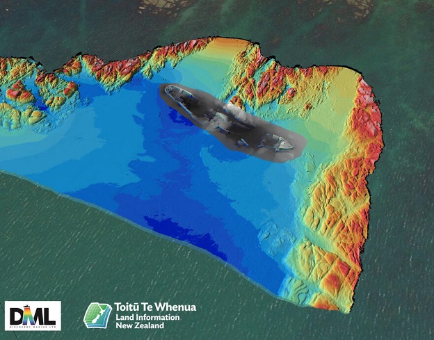
The first is bathymetric data, which provide a three-dimensional map of the surface of the seafloor.
The second is seismic data, which provide information on the depth, thickness, and other characteristics of the sediments beneath the seafloor.
Geological samples and other geophysical techniques, where available, are used to augment these primary data types.
U.S. data collection began in 2003 and constitutes the largest offshore mapping effort ever conducted by the United States.

Who did the work?
The ECS Task Force, an interagency body of the U.S. Government, coordinated the delineation of the outer limits of the U.S. ECS.
The Department of State chairs the Task Force, leads the ECS Project Office, and manages the project’s diplomatic and legal aspects.
The U.S. Geological Survey (USGS) leads the effort to collect, process, and interpret the seismic and geologic data.
The National Oceanic and Atmospheric Administration (NOAA) leads the effort to collect, process, and analyze the bathymetric data.
Many other Federal and academic partners collaborated to complete the work over the course of more than 20 years.

Is the United States extending its exclusive economic zone (EEZ)? 
No. The ECS is not an extension of the EEZ.
The continental shelf includes only the seabed and subsoil, whereas the EEZ also includes the water column.
In addition, while the maximum extent of the EEZ is 200 nautical miles from the coast, the continental shelf may extend beyond 200 nautical miles.
Some of the rights that a country has in its EEZ, especially sovereign rights over water column resources (such as fish), do not apply to the ECS.

Does the U.S. ECS overlap with the ECS areas of any neighboring countries?
Yes. The U.S. ECS partially overlaps with ECS areas of Canada, The Bahamas, and Japan.
In these areas, the United States and its neighbors will need to establish maritime boundaries in the future.
In other areas, the United States has already established ECS boundaries with its neighbors, including with Cuba, Mexico, and Russia.

Does the Administration still support joining the Law of the Sea Convention?
Yes. Like past Administrations, both Republican and Democratic, this Administration supports the United States joining the 1982 UN Convention on the Law of the Sea.
The announcement of the U.S. ECS limits in no way changes the Administration’s position toward the Convention.  
 
Links :
 

Thursday, December 21, 2023

One woman makes history at the helm in 1856

 
From FreghtWaves by Brielle Jaekel
 
When the captain of an American merchant ship fell ill, his wife took command

Mary Ann Brown married Joshua Adams Patten before she turned 16.
He was captain of a ship named Neptune’s Car, owned by Foster & Nickerson, according to an article from the New York Tribune
After their marriage, she joined him on the ship for a journey that lasted 17 months and took them from New York to San Francisco, China, London and back to New York.
Mary Patten helped pass the time by studying navigation.

This pastime would become more important than she ever could have predicted.
 

In 1856, a 19-year-old pregnant woman by the name of Mary Ann Brown Patten took command of an American merchant vessel named Neptune's Car when the captain (her husband) developed tuberculosis and fell into a coma.
Usually in such a case, the first mate would have assumed command of the vessel. However, the first mate had been locked up in his cabin after it was discovered that he had been purposely slowing down the vessel because he had taken bets on a competitor vessel.
As for the second mate, he was an illiterate man who was unable to navigate.
For 56 days, Mary Ann took the helm of Neptune's Car and was able to bring it safely to San Francisco despite a mutiny to overthrow her.
During the voyage, the first mate demanded that Mary Ann release him immediately and reinstate him as commander of the vessel.
However, she refused.
The first mate then tried to instigate a mutiny, but Mary Ann was able to convince the crew to stick by her side and eventually won their unanimous support. 
Mary Ann did not change her clothes for 50 days and during her spare time, studied medicine in order to take care of her husband.
While his health never fully recovered, Mary Ann managed to keep him alive for the duration of the trip.
When the insurers of the ship rewarded Mary Ann with a $1,000 gift, she replied in a letter that she was doing "only the plain duty of a wife."

A history-making journey

Capt. Patten was commissioned to again command Neptune’s Car from New York to San Francisco in 1856.
Mary, now 19, was four months pregnant but still joined her husband for the voyage.

The navigational skills she had acquired proved vital when Capt. Patten developed a high fever and fell gravely ill.
Mary Patten became the ship’s commander and navigated the vessel on its difficult journey, which included sailing around Cape Horn, according to WomenOffshore.org.
 
The journey was not easy and Mary Patten faced a lot of difficulties.
While she was in command of the ship, she also tended to her husband’s illness.
And as Mary Patten battled rough seas and her husband’s worsening condition, another problem was brewing.

Early in the voyage, the first mate, whose name has been lost to history, reportedly fell asleep while on watch and was fired by the captain.
Yet he remained onboard Neptune’s Car.
Said to be angry about his circumstances and distrustful of a woman in command, he began to plan a mutiny.

The former first mate insisted on changing course and abandoning the trip to San Francisco, according to the New York Tribune article, which said Capt. Patten relayed his disagreement from his chambers and continued to put his faith in his wife.
The crew reportedly was also confident in Mrs. Patten’s abilities and rallied behind her, successfully quashing any attempted mutiny.

After 120 days, Neptune’s Car made its arrival in San Francisco.
The owners of the ship awarded Mary Patten $1,000 for her service in delivering the crew and cargo safely, according to WomenOffshore.org.

In an interview with the New York Tribune following the harrowing journey, Mary Patten revealed she had not changed out of her clothes for 50 days in order to maintain her duties.
She expressed a desire to be excused from talking about herself and claimed she had only done her duty as a wife.
She also disclosed that her husband had lost his sight and hearing to the sickness.

Mary Patten gave birth to her son a few months later, and Capt. Patten passed away from his illness three months after that.
 
Links :

Wednesday, December 20, 2023

How good are long-range forecasts?

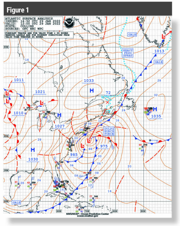
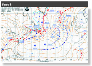
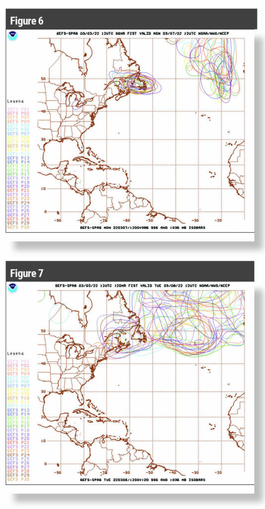
Voyagers rely on long-range forecasts to find the right weather window for a passage.

From Ocean Navigator by Ken McKinley is a weather professional and vessel router who owns Locus Weather (www.locusweather.com) in Camden, Maine.

Examining a recent Atlantic storm offers some insight

Ocean-going mariners have many sources for weather forecast information these days, and thanks to the internet and satellite communication technologies, these resources are readily available both ashore and at sea.
Improvements in the science of weather forecasting have allowed longer and longer-range forecasts to be produced in recent years to the point that 96- and 120-hour (four- and five-day) forecasts are now routinely available, and even longer range forecast information can be accessed.
But it is worth asking the question: How reliable are these forecasts?

To answer this question, let’s look at a recent situation.
 
Figure 1: Surface pressure analysis for the morning of Jan.
29, 2022.


The northeastern U.S. and Atlantic Canada were hit with a powerful nor’easter in late January of 2022.
This system produced large amounts of snow and also generated very strong winds both over land areas and over the ocean.
Figure 1 is the surface pressure analysis chart which shows this system on the morning of January 29, 2022.
The strong winds from this system resulted in very high seas over coastal and offshore waters with significant wave heights up to 26 feet east of New Jersey at 1200 UTC January 29, and up to 35 feet east of southern New England 12 hours later at 0000 UTC January 30.

This system was generally very well forecast.
Media reports for many days prior to the arrival of the system were highlighting the possibility of a major storm, and weather forecasts, both the official government forecasts, and those produced by the media, were quite accurate in describing the impacts of the storm.
Often the hype in advance of significant weather events can be over the top, but in this case it was generally justified.
This does not mean that all forecast parameters were perfect for all locations — that is a standard that is rarely met — but the forecasts available to the public provided a very good picture of conditions produced by this system well in advance.

This is rather remarkable given the fact that an identifiable low-pressure center at the surface was not present for this system 24 hours before the time of Figure 1.
Forecasters of a couple of generations ago likely would have had the ability to predict the development of this storm based on upper-level weather patterns a couple of days in advance.
It would have been difficult, however, to predict the intensity of the system, and an accurate forecast for such a system more than about three days in advance would most likely not have been possible.
 
 
Figure 2 is the 96-hour surface forecast chart valid for same time as figure 1.

Long-range forecasts

Figure 2 shows the 96-hour surface forecast chart valid at the same time as Figure 1.
This chart, which was generated four days before the system was impacting the northeastern U.S.
and the adjacent Atlantic, forecast that the low would be located a bit farther south than where it ended up, and that its central pressure would not be quite as low.
Figure 3 shows the 96-hour forecast that was produced 24 hours earlier than Figure 2.
There is no significant low forecast to be present in the eastern U.S.
or over the adjacent Atlantic at the valid time of this chart, but the arrow in the western Atlantic does indicate a low forecast to develop after the valid time of the chart, showing a forecast center position 24 hours after the valid time of the chart (the same time as Figures 1 and 2) at about 37° N/70° W and a forecast central pressure of 980 millibars.
The term “rapidly intensifying” on the chart indicates that the central pressure of a low is forecast to drop at least 24 millibars in a 24-hour period, the criteria for a “bomb cyclone.”
 
  
Figure 3 is the 96-hour forecast chart for 24 hours earlier than the figure 2 chart.

While neither of these 96-hour forecasts were perfect, they were both remarkably good for a system like this, providing five days of notice that there would be an impactful storm affecting this region.
Thus, for this system, the long-range forecasts were extremely accurate and very useful.

Let’s dig a little deeper as to the origin of this system.
Mid-latitude lows like this one are powered by energy in the upper levels of the atmosphere which is often best represented by looking at waves in the 500-millibar flow.
Much like waves on the surface of the ocean, waves in the atmosphere can grow, or amplify with time, but can also flatten out, or weaken with time.
Also, like ocean waves, there are bigger waves and smaller waves, and they all interact with one another, sometimes combining to produce a really big wave, and at other times interacting in a way that leads to waves becoming less prominent with time.
 
 
Four views of the 500-millibar chart showing a trough over the Aleutian Islands sweeping east to the eastern US and supporting the development of the strong nor’easter.

Figure 4 shows 500 millibar analyses across a good portion of the northern hemisphere for selected days in the week leading up to the nor’easter.
Examining the final panel of Figure 4, which is the 500 mb analysis valid at the same time as Figure 1when the nor’-easter was well developed as a powerful storm in the western Atlantic, one can plainly see a well-developed, high amplitude wave in the 500-millibar flow over the eastern U.S.
This is termed an upper level trough, and the red line shows the rough axis of the trough.
Strong surface lows are typically found downstream of 500-millibar trough axes during their developing phase, and this was certainly the case in this situation.
Then, by working backwards in time, one can see where this trough axis was located in the days leading up to January 29, 2022.

The first panel in Figure 4 was valid on Monday January 24, 2022, and this is the actual data from which the 96-hour forecast shown in Figure 3 was generated.
It is remarkable that forecasting skill has evolved to the point that a somewhat nondescript 500-millibar trough that extended from the upper Aleutian Islands south toward Hawaii was able to be forecast to develop into a very strong mid latitude low in the western Atlantic five days later with such precision.

The second panel in Figure 4 was valid the next day (Tuesday January 25, 2022).
This is the actual data from which the 96-hour forecast, shown in Figure 2, was generated.
Again, this trough, then located
to have higher confidence in the prediction.
The third panel of Figure 4 (valid two days after the second panel) shows that the 500-millibar trough has progressed up and over the upper level ridge over the western U.S.
and has begun to amplify as it nears the central U.S., and it is well on its way to supporting the development of the strong nor’easter.

The example of this nor’easter is clearly a situation where the long-range forecast was very good, perhaps even excellent.
Even though every forecast is not as accurate as this one, studies generally show that forecasting skill has improved significantly over the past few decades.
Much of this improvement can be linked to the advances in the computer models to the point that forecasts of conditions four to five days ahead are quite reliable, as in this case.
At times, though, situations can exist where forecasts of this range are not as successful.
This can be traced to several possible issues, including poor initial data, particularly over data-sparse areas of the planet (like open ocean areas), wave patterns that are unstable or cannot be well resolved in the initial data, and shortcomings in the forecast models.

Ensemble forecasts

Another tool which has come into more common use in recent years is the ensemble forecasting method.
This involves acknowledging that the initial data may not be completely accurate and running a model multiple times with very slight changes in the initial data field.
The idea behind the concept is that if the pattern is generally more predictable, then the slight changes in the initial data field will not make much difference, and the model will tend to converge on the same forecast output at a given future time.
On the other hand, if the pattern includes elements that are less able to be accurately forecast (perhaps small-scale features that cannot be well defined are present, or the model may have difficulty capturing how the different scales of waves will interact with one another) then the small changes made in the initial conditions will lead to very different outputs as time is stepped forward in the model.
This allows the forecaster to be more (or less) confident in the results of each model run.

The general public is used to seeing deterministic forecast products, which in the case of forecast charts means that the forecaster must state that, for example, a low-pressure center will be in a certain position at a given future time, and that it will have a specific central pressure value.
The 96-hour forecasts shown in Figures 2 and 3 are examples of deterministic forecast products.
But the reality of meteorology is that forecasting is often more probabilistic in nature, with multiple outcomes possible given an initial pattern and our current knowledge of the atmosphere.
The ensemble technique is able to help assess the probability of possible different future outcomes of certain weather fields, like the 500-millibar pattern or the surface pressure pattern.
The forecasters at the NOAA’s Ocean Prediction Center have access to the ensemble forecast fields, and this can help them to come up with the most reasonable deterministic forecast at a given time.
 
 
Figure 5 shows a 96-hour surface forecast for March 7, 2022.

Figure 5 shows a 96-hour surface forecast valid at 1200 UTC on March 7, 2022.
Figure 6 is an example of ensemble forecast output from the same forecast cycle, valid at the same time.
There are 30 ensemble “members”, which represent 30 different tweaks to the observed data set that initialized this model run.
In this depiction, only one isobar is shown (996 millibars), but it is shown for every ensemble member.
These charts are sometimes referred to as “spaghetti plots.” Notice that the collection of isobars (ensemble members) around Newfoundland and Atlantic Canada shows some variation, but not a lot.
This allows the forecaster preparing the chart in Figure 5 to be fairly confident in the placement of a low in that region.
Looking farther east, though, there is quite a bit more variation in the ensemble members of the isobars, suggesting more computational instability in the pressure fields generated by the model for this region, and this means that the placement of the low on the forecast chart has a lower probability of being correct when the actual time arrives.
There is no indication of this lower probability on the deterministic forecast chart, though, as the forecaster must make the best decision possible for the forecast location and strength of this low in the eastern Atlantic.
 
 
Figure 6 and figure 7 are ensemble forecasts that contain 30 ensemble “members.”

Figure 7 is the ensemble model data from the same model run and for the same isobaric value, but it is valid 24 hours later.
This clearly shows that this data set becomes more computationally unstable for the later forecast time.
This means that the arrows showing the movement and forecast central pressures of the lows on the 96-hour forecast chart (Figure 5) have a lower probability of ultimately being correct.

Weather apps and forecasts

There are many weather apps available to mariners that provide forecasts of several different parameters, and these apps generally present output from forecast models without any input from human forecasters.
The models that are used most frequently are the US-based GFS model, and the European-based ECMWF model.
Questions are often asked as to which model is better, but there is no one set answer to this as the models will perform differently in different weather patterns, and sometimes one will provide a better forecast, and sometimes the other will be superior.
Sometimes these two models will show significantly different forecasts, particularly in the longer-range time periods.
When this occurs, it is an indication that the existing weather pattern does not lend itself well to being predicted by the mathematical models.
When these two models show similar forecasts, the confidence level in their forecasts is increased.

The answer to the question initially posed is that forecasts in the four- and five-day range are generally quite good and can be used reliably to make decisions about ocean voyages.
But they are not perfect, and forecast data generally becomes less reliable for longer ranges.
As noted above, some weather patterns are more predictable than others, and the ensemble forecast data offers a window into this situation.
This data can be found through NOAA’s Model Analyses and Guidance web page (mag.ncep.noaa.gov).
Those mariners who have access to data from different models through apps (often termed GRIB data) should interpret differences in the model output as an indication of a lower probability forecast, and should consider that all possible outcomes are possible, and plans should be made with that in mind.

Another strategy that should be employed by mariners is to pay attention to how the model (GRIB) data changes in successive model runs.
Again, if there is consistency from run to run, this generally suggests a higher confidence level in the forecast output.

Keep in mind that weather apps providing GRIB model output are just tools, and it is always best to use them in combination with forecasts produced by professional meteorologists.
This includes forecasts available through NOAA’s Ocean Prediction Center.

The meteorologists who generate these forecasts have access to everything that a mariner may see in an app, and obviously much more as well.
These additional resources including model data from several models, ensemble plots, and they may also have information about any shortcomings in the initial data set for each forecast cycle.

Professional meteorologists use this data along with their knowledge and experience to produce with the best deterministic forecasts possible.
The end result is steadily improving long-range forecasts. 

Links :

Tuesday, December 19, 2023

Two maps show why shipping firms are suspending routes in the Red Sea


From Washington Post by Laris Karklis
 
This month at least six commercial ships traveling through the Red Sea have been subjected to drone and missile attacks as they approached the narrow Bab el-Mandeb Strait.
The attacks have come from Iranian-backed Houthi rebels, who since 2014 have controlled a large portion of western Yemen, including the capital, Sanaa, and coastal areas along the Red Sea.
 
Armed men stand on the beach as the Galaxy Leader commercial ship, seized by Yemen's Houthis last month, is anchored off the coast of al-Salif, Yemen, on December 5, 2023
[Khaled Abdullah/Reuters]

The attacks endanger ships traveling through this vital corridor from the Suez Canal through the Indian Ocean with cargo and energy shipments .
The Houthis have claimed that these attacks are aimed at ending the Israeli air and ground offensive targeting the Gaza Strip and Hamas.

The Red Sea is defined by two narrow waterways: to the north, the Suez Canal, an Egyptian waterway; and to the south, the Bab el-Mandeb Strait.
The strait is only 20 miles wide and is bordered by Djibouti and Eritrea to the west and Yemen to the east.
Nearly 10 percent of all oil traded at sea passes through it, and an estimated $1 trillion in goods moves through the strait annually.
The Strait of Hormuz, which is the entryway to the Persian Gulf and is bordered by Iran and Oman, is roughly 30 miles wide, for comparison.

MarineTracker, a company that tracks global shipping, indicated that one of the ships reportedly attacked Friday, the MSC Palatium III, passed through the strait and upon being attacked turned around rather than continue north closer to the rebel-held coast.
 
Amidst the maritime chaos unfolding in the Red Sea, here is a simple graphic detailing recent incidents in Bab-el-Mandeb region, this visual encapsulates current challenges faced by one of the globe's busiest shipping routes

Bab al-Mandeb Strait chokepoint


On Friday, one day after an aerial missile narrowly missed a Maersk ship, the Gibraltar, the Danish shipping company instructed all Maersk vessels bound to pass through the Bab el-Mandeb Strait to pause their journeys until further notice.
Another shipping company, the German-based Hapag-Lloyd, also suspended container traffic through Monday.
 
The US Navy Arleigh Burke-class, guided-missile destroyer USS Carney has been intercepting drones and missiles in the Bab al-Mandab Strait in recent months
[Reuters]

Maersk, posting on X, said that “the recent attacks on commercial vessels in the Bab al-Mandab Strait are alarming and pose a significant threat to the safety & lives of seafarers. … 
This issue cannot be addressed by the global shipping industry alone, and we urge the international society to come together to find a swift resolution to bring the situation under control.”

U.S. national security adviser Jake Sullivan said in Tel Aviv on Friday that the United States is “building a coalition” and will take “every step” to deter the Houthi rebels from carrying out attacks in the Red Sea.

Links :

Monday, December 18, 2023

Uncharted NZ shipwrecks mapped for first time

3D image of the Star of Canada wreck captured a LINZ hydrographic survey.
 
From SpatialSource by J. Nally
 
Two previously uncharted shipwrecks have been revealed and mapped during a hydrographic survey of Tūranganui-a-Kiwa/Poverty Bay, in the Gisborne region on the north-eastern coast of New Zealand’s North Island.
 
Localization with the GeoGarage platform (Linz nautical raster chart)

The Toitū Te Whenua Land Information New Zealand (LINZ) survey of the Gisborne area uncovered the vessels: the hull and deck structure of the 7280-tonne steamer Star of Canada, which ran aground off Kaiti Beach on 23 June 1912, and the wreck of a barge used to dredge Napier and Gisborne harbours in the 1930s.

“It’s always satisfying when our surveys reveal features that were either unknown or uncharted,” said LINZ Principal Geospatial Specialist Stuart Caie.
“Advances in technology mean that each time we resurvey an area we uncover details that were previously unknown. In this case, the last survey was done in the 1950s by the Navy and the echosounding technology used this time has given us far greater coverage of the seafloor than ever before.
“While the local community is aware of these wrecks, they have never been charted.”

Another 3D image of the Star of Canada wreck.

The Star of Canada regularly sailed from Australia and New Zealand to England between 1910 and 1912, carrying chilled and frozen meat and other produce.

On 23 June 1912, a squall blew the vessel onto Kaiti Beach where it grounded just off the rocky shoreline and began taking on water.
 
Localization with the GeoGarage platform (Linz nautical raster chart)
 
Fortunately, no lives were lost, but the vessel had to be abandoned
 

The Star of Canada seen as it was the process of slowly sinking.
Image credit: Auckland Libraries Heritage Collections NZG-19120710-0027-01.

The other wreck comprises the remains of the dredge Korua, which was scuttled off Young Nick’s Head when it was no longer of use.
 
Black and white image of the dredge KORUA

Data captured in the overall survey, including details of the wrecks, will be used to update nautical charts of the area.

3D image of the dredge Korua in fragments on the seafloor.
 
Links :

Sunday, December 17, 2023

Discover the Arcachon whale tail, an unusual beacon...

 
From BoatNews by Maxime Leriche
 
Every spring, a new species of marine mammal takes up summer residence off the coast of Arcachon.
Installed between the Thiers and Eyrac jetties, this whale tail is actually a floating work of art, with a new decoration every year.
We spoke to Emmanuel Janssens Casteels, the artist behind this marine work of art.


A local initiative

The Arcachon whale tail was created in 2010 by Emmanuel Janssens Casteels, a Belgian artist specializing in life-size reconstructions in the natural sciences.
His creations are usually destined for museums, cinema or scientific purposes.
He was kind enough to tell us about the genesis of this highly original project:
"I was asked by the Arcachon town council to design an ephemeral work. I suggested a whale's tail in the process of sounding. The town council found the idea excellent and quickly approved the project. I was lucky enough to have a cast of a real whale tail in my studio. I tested it in a 3m prototype pool to validate the calculations". 
 
Localization with the GeoGarage platform (SHOM nautical raster chart)

Polyester construction 


It was in his workshop in Prayssas, in the Lot et Garonne region, a long way from the sea, that the whale tail was made.
It took over 6 months of hard work to complete the project, as Emmanuel explains:

"After conclusive tests, we set about building this 9.6-metre span, almost 10-metre high structure. To build it, I created large templates, with a polyester envelope, a bit like making a boat hull. The counterweight is made of stainless steel. I redesigned the silhouette to resemble a whale's tail, with stiffeners to guarantee the curves.

The transport was done in several pieces.
I assembled everything in the technical area of the port of Arcachon.
With a draught of 5m, the whole thing weighs almost 2 tonnes. 


When it was launched, I was a bit worried that it wouldn't work. I'm not used to floating structures. Initially, the project was supposed to last just one season.
But in the end, the structure held firm, and the whale tail has now been on display on Arcachon's beaches every summer for almost 13 years".

Moored on a solid mooring, she's in the water from spring to early autumn, and takes shelter every winter near l'Aiguillon. 
 

New colors at every launch 


Since its launch in 2011, the Arcachon whale tail has changed color with each new tourist season.
These new colors are chosen according to an event or current trends, and are a delight for tourists. 


Recently, an autumnal depression hit the basin, and the whale tail broke its mooring, wandering to the bottom of the basin.
Stranded on a sandbank, it has since returned to its winter home to refresh itself before the next season.