Saturday, February 21, 2015

Coral city


Take an exclusive look at the process behind Coral Morphologic's living artworks, colorful reefs created using coral polyps native to Miami.
Watch as the scientific art collective explores the visual storytelling potential of coral reef organisms through film, multimedia and site-specific artworks.
Additionally, learn how rising sea levels, combined with government dredging projects, are impacting not only corals, but the entire fate of Miami.

Friday, February 20, 2015

Mapping landscapes in the deep ocean

Researchers at the National Oceanography Centre (NOC) have developed a new, automated method for classifying hundreds of kilometres of the deep sea floor, in a way that is more cost efficient, quicker and more objective than previously possible.

From NOC

Currently there is very little information about the geographic distribution of life on the sea floor.
This is largely because of the practical difficulty in accessing creatures which live at such a great depth in the ocean.
However, this research soon to be published in the journal Marine Geology, reveals a new method of estimating this distribution using a combination of: submarine mapping technology, statistics and a ‘landscape’ ecology technique called ‘Niche Theory’, which is generally used on land.

The Niche Theory states that biodiversity is driven by spatial variability in environmental conditions, i.e. the greater the range of habitats, the greater the biodiversity.
The lead author of this study, Khaira Ismail from the University of Southampton, has used this concept to create broad-scale, full coverage maps of the sea floor.
The objective of these maps is to estimate the location of biodiversity hotspots, by identifying areas where the deep-sea landscapes are relatively more varied.


Bathymetry map of Lisbon–Setúbal and Cascais Canyons offshore Portugal, overlain by TOBI sidescan sonar imagery coverage.
Contour interval is 500 m.
The inset map shows the location of the study area relative to the location of Portugal.

Dr Veerle Huvenne, from the NOC, said “by informing us of where to look and where to plan more detailed surveys, this new method will help to make our deep-sea research more targeted and efficient, by advancing our understanding of life in the deep ocean, which at the moment is still very limited.”

These maps cover areas approximately 200km across, and have pixel sizes around 25m.
They are created using information on the topography and sediment type of the sea floor, collected from a multi-beam echo sounder and a side scan sonar, respectively.
The resulting map is then analysed in order to break down the sea floor into a series of zones, using statistical analysis to identify distinct ‘geomorphological terrains’ in an objective and repeatable way.


3D views of the Portuguese Canyons from south.
The figure shows variations of bathymetric position index analysis (top) and slope analysis (bottom) resulting from using two different length scales.
The local length scale is 25 m (initial pixel size) and broad length scale at 225 m.
Note the different features delineated at the different analysis scales.
Results from local length scale contained detail features but noisier whereas broader length scale shows the gross canyon morphology.

Khaira said “using statistical methods to identify these ‘terrain zones’ allows us to be more objective than if we were picking them out by hand.
This objectivity means that the results are consistent and repeatable, which allows different areas of the sea floor to be compared more easily.”


An expert visual interpretation of Setúbal Canyon from sidescan sonar imagery collected in 2005 used for visual comparison with automated marine landscape map.
A, B, C, and D are zoomed figures of the visual interpretation map from sidescan sonar imagery (left) in the selected area (outline in black) compared to automated marine landscape map (right).
 The expert interpretation in this area lacked contiguity and coverage, although manual delineation allows individual features to be picked out there is always a possibility of it being missed due to human error. In comparison, the automated technique produced a more consistent map but often too generalized (i.e.: small features are often grouped together).

This research forms part of the €1.4M European Research Council funded CODEMAP project, and was applied in the Lisbon-Setúbal and Cascais Canyons, off the Portuguese coast.
These submarine canyons were classified into six marine ‘seascapes’, based on their geomorphological features.

Future work will use submarine robot cameras to take photos and videos of life in the deep-sea areas that have been subjected to this mapping technique.
This will allow researchers to start to identify new deep sea habitats.

Thursday, February 19, 2015

Image of the week : new land on the Louisiana Coast

acquired November 7, 1984

acquired October 25, 2014

 Atchafalaya Bay with the Marine GeoGarage

overlayed on Google imagery (09/2014)

From NASA

While most of the delta plain of the Mississippi River Delta is losing ground, new land is forming in Atchafalaya Bay at the mouths of the Wax Lake Outlet and the Atchafalaya River.
Geologists first noticed mud deposits building up in Atchafalaya Bay in the 1950s, but new land first rose above the water line in 1973 after a severe flood.
Since then, both deltas have grown considerably. According to one estimate by scientists from Louisiana State University (LSU), the Atchafalaya and Wax Lake Outlet deltas have combined to grow by 2.8 square kilometers (1 square mile) per year.

This pair of false-color satellite images illustrates the growth of the two deltas between 1984 (top) and 2014 (bottom).
Both images were acquired by sensors aboard Landsat satellites.
A combination of shortwave infrared, near infrared, and green light was used to accentuate differences between land and water.
Water appears dark blue; vegetation is green; bare ground is pink.
All of the images were acquired in autumn, when river discharge tends to be low.
Vegetation appears slightly brown in 1984 because the image was acquired later in the year.
Use the image comparison tool to slide between the two images.

The Atchafalaya is a distributary of the Mississippi River that connects to the “Big Muddy” in south central Louisiana near Simmesport.
Wax Lake Outlet, an artificial channel designed to reduce the severity of floods in Morgan City, delivers about 40 percent of the Atchafalaya’s water into the bay about 16 kilometers (10 miles) west of where the main river empties.

The deltas’ rate of growth has varied considerably, mainly due to the timing of major floods and hurricanes.
Floods transport large volumes of extra sediment to Atchafalaya Bay, while hurricanes redistribute sediment within the bay and transport it offshore into deeper waters.
Hurricanes also destroy coastal vegetation that would otherwise protect land from erosion.

The Atchafalaya delta has grown at a faster rate than its neighbor—about 1.6 (0.6 square miles) square kilometers per year, versus 1.2 square kilometers (0.46 square miles) per year for the Wax Lake delta.
The difference is due to regular dredging and channel widening on the lower Atchafalaya, which delivers extra sediment to its delta.
Due to the lack of dredging, Wax Lake delta is more natural in character, with a more symmetric, lobate shape.

“We are looking carefully at the Wax Lake and Atchafalaya deltas as models for building new land and preserving some of our coastal marshlands,” said Harry Roberts, director of the Coastal Studies Institute at LSU.
“If we start diverting significant portions of the water and sediment from the main channel of the Mississippi River into adjacent wetlands, lakes, and bays—as happens now in Atchafalaya Bay—we’ll be taking an important first step toward saving a significant part of Louisiana’s coastal plain.”

Learn more and see more imagery by reading “Growing Deltas in Atchafalaya Bay.”

Wednesday, February 18, 2015

Researchers propose high seas fishing ban

Based on a scenario where the catch of straddling taxa increase by 18% following a high-seas closure. Current landed value is the product of catch and ex-vessel price.
Catch data were extracted from the Sea Around Us global catch database26 (www.seaaroundus.org) while ex-vessel prices were obtained from Sumaila et al.29 and Swartz et al.19.
The annual catch of straddling taxa by each fishing country was projected to increase by 18% under the high-seas closure scenario, whereas the catch of non-straddling taxa remains unchanged. Countries with negative and positive change in landed values were labelled “Loss” and “Gain” in the map, respectively.

From FIS

Closing the high seas to commercial fishing could distribute fisheries income more equitably among the world's maritime nations, according to research from the University of British Columbia (UBC).

The analysis of fisheries data indicates that if increased spillover of fish stocks from protected international waters were to boost coastal catches by 18 per cent, current global catches would be maintained.
When the researchers modelled less conservative estimates of stock spillover, catches in coastal waters surpassed current global levels.

Fishing vessel in high seas

The study examined global fish catch and landed value data to determine how much fish is caught in the high seas and how much is caught in coastal waters (nations' 200-mile exclusive economic zones).
The researchers then used models to compare likely increases in coastal catches driven by increased biomass spillover from protected areas and losses from the closure of high seas fisheries.

“We should use international waters as the world's fish bank,” says Rashid Sumaila, director of the UBC Fisheries Economics Research Unit and lead author of the study.
“Restricting fisheries activities to coastal waters is economically and environmentally sensible, particularly as the industry faces diminishing returns.”

 Fishing in Iceland waters in the North Atlantic.
Big catch of red fish hauled on board a freezing trawler.

The findings appeared yesterday in Scientific Reports, published by Nature Publishing Group and will be presented today at the 2015 annual meeting of the American Association for the Advancement of Science (AAAS).

Average annual portions of taxa taken from the high seas only, from both the high seas and Exclusive Economic Zones (EEZs), and from EEZs only based on global catch statistics 2000–2010.

The study also indicates that a high-seas moratorium would improve fisheries income distribution among maritime nations.
Currently, 10 high seas fishing nations capture 71 per cent of the landed value of catches in international waters.

Under all scenarios considered by the researchers, European Member States, Group of Eight nations, and least developed fishing nations would benefit the most from a closure.
Under a catch-neutral scenario, the United States, Guam and the United Kingdom would benefit the most, each with potential increases in landed values of more than USD 250 million per year.
Canada would see an increase of USD 125 million annually.

Supertrawlers like the FV Margiris set to be banned from Australian waters permanently

While closing the high seas would benefit some countries, others stand to lose significant fisheries income. South Korea, Taiwan and Japan would each see a decrease in catch values of at least USD 800 million per year in a catch-neutral scenario.
Countries that sail vessels under flags of convenience would also be hard hit.
While this figure is not insignificant, Sumaila points out that the high seas belong to the world and currently only a few countries benefit from the fish resources.
Countries fishing in the high seas will have to give something up to achieve higher levels of food security and profits globally.

The authors acknowledge that implementing a high seas ban would be a major undertaking, but argue that the ongoing expansion of human activities into the oceans may soon require major reform to the governance of international waters, while penalties imposed on illegal fishing could offset administrative and operational costs.

Tuesday, February 17, 2015

Satellite images to monitor ocean acidification in remote areas from space


Five years of global sea-surface salinity from space
Variations in 10-day mean sea-surface salinity derived from SMOS data
over a five-year period on a grid resolution of 0.5 x 0.5°.
Nicolas Reul (Ifremer)

From RT

A group of international researchers is developing "pioneering techniques" to monitor the acidity of oceans from space, using satellites that can orbit the Earth up to 700 km above us in hard-to-reach areas, like the Arctic, much faster than before.

 Scientists have used satellite data to map the alkalinity of the world's oceans for the first time.
The image above shows the average level of alkalinity over the past five years with blue marking water that is more acidic.
By using satellite data, scientists can obtain live information as the ocean changes

According to the scientists, a number of existing satellites can be used for the task, including the European Space Agency's Soil Moisture and Ocean Salinity (SMOS) sensor that was launched in 2009 and NASA's Aquarius satellite launched in 2011.

"Satellites are likely to become increasingly important for the monitoring of ocean acidification, especially in remote and often dangerous waters like the Arctic.
It can be both difficult and expensive to take year-round direct measurements in such inaccessible locations," said lead researcher Dr Jamie Shutler, of the University of Exeter.
"We are pioneering these techniques so that we can monitor large areas of the Earth's oceans allowing us to quickly and easily identify those areas most at risk from the increasing acidification," he said.

 Sea-surface salinity and ocean circulation
Average sea-surface salinity values.
Areas of red indicate regions of high salinity, and areas of green indicate regions of low salinity.
The map is overlaid with the simplified global circulation pattern called the ‘thermohaline circulation’.
The blue arrows indicate cool deeper currents and the red indicate warmer surface currents.
Temperature (thermal) and salinity (haline) variations are key variables affecting ocean circulation.

Each year, over a quarter of global CO2 (carbon dioxide) emissions from burning fossil fuels and cement production are absorbed by the planet's oceans.
This process makes the seawater become more acidic and as a result more difficult for some marine life to exist.
Growing CO2 emissions, along with the rising acidity of seawater, could devastate some marine ecosystems over the next century, ecologists warn, and that's why endless monitoring of changes in ocean acidity is vital.
A report issued before a United Nations climate summit in New York put 2014 world carbon emissions 65 percent above levels in 1990, despite repeated promises of curbs and a shift to renewable energies.
It said world emissions could reach 43.2 billion tons in 2019, with 12.7 billion from China alone, as the number one carbon emitter.

 Global salinity maps from SMOS (ESA/IFREMER)

Current methods of measuring temperature and salinity to determine acidity are restricted to in situ tools and measurements from research vessels.
Since such vessels are expensive to run and operate, the approach limits the sampling only to small areas of the ocean, however.

The groundbreaking techniques use satellite mounted thermal cameras to take ocean temperatures, while microwave sensors check salinity.
These measurements can be used to assess ocean acidification more quickly and over much larger areas than has been possible before, researchers say.

"In recent years, great advances have been made in the global provision of satellite and in situ data.
It is now time to evaluate how to make the most of these new data sources to help us monitor ocean acidification, and to establish where satellite data can make the best contribution," said Dr Peter Land from Plymouth Marine Laboratory, the lead author of the paper, set to be published on Tuesday in the journal Environmental Science and Technology.

Scientists from the University of Exeter, Plymouth Marine Laboratory, Institut français de recherche pour l'exploitation de la mer (Ifremer) and the European Space Agency took part in the research.

Links :

Monday, February 16, 2015

Maps provide another view of South Florida history

The government's first nautical map of South Florida (1855)
showed most of the development was south of the Miami River.
(NOAA Office of Coast Survey)

 South Florida in 2015 with the Marine GeoGarage

From Sun Sentinel by Ken Kayle

In 1854, six years before the Civil War, the U.S. government first mapped the South Florida coastline, primarily to mark the depth of shoreline waters and prevent ships from breaking up on rocks.
The map didn't show much other than obscure landmarks such as Turkey Point, a place that actually had turkeys, not a nuclear plant.
Over the decades, updated maps were produced, depicting the rapid buildup of the coastline and providing another view of history.
Now, you can see it for yourself, free of charge.
The National Oceanic and Atmospheric Administration's Office of Coast Survey has put all its maps on its online site – historicalcharts.noaa.gov.

"You see the progression of coastal changes," said agency spokeswoman Dawn Forsythe.
"You can match them up and compare them with today's charts."
For instance, the 1855 map shows the bulk of South Florida's population was south of the Miami River, in what is now downtown Miami.
Aside from Virginia Key and Key Biscayne, most of the landmarks had unfamiliar names, such as Shoal Point, Black Point and Elliott's Beach.

 Here's the nautical map for Fort Lauderdale in 1895.

 Fort Lauderdale with the Marine GeoGarage in 2015

Four decades later, in 1895, a map indicated development was spreading north.
The Fort Lauderdale area is shown having two settlements, Lauderdale and Cocoa Palms, near what is now Sunrise Boulevard.
By 1927, Miami, Fort Lauderdale and West Palm Beach already were fairly well developed. However, Port Everglades still was Lake Mabel, three to six feet deep with a rocky bottom.
By 1951, maps show the entire South Florida coastline was burgeoning with cities, canal systems, ports, isles, bridges, tall buildings and docks.

That was the result of a land boom, said Debi Murray, chief curator of the Historical Society of Palm Beach County.
"The early 20th Century was a period of huge growth because of the Flagler railroad and because people started selling lots like crazy," she said.
Something the maps don't clearly depict: How two Category 4 hurricanes, in 1926 and 1928, devastated the region for years.

The maps prior to those storms show South Florida's cities having simple street grids and little coastal development.
Yet by the mid 1930s, maps show Miami, Fort Lauderdale and Miami flourishing with swing bridges, a network of waterways, yacht clubs, radio towers and water tanks.
In between, the region suffered miserably, Murray said.
"The 1926 hurricane put the brakes on growth and widely affect the entire region," she said.
"The 1928 hurricane destroyed thousands of homes and killed between 3,000 and 3,200 people – and we were already in a local recession then."
What rescued the region was President Franklin D. Roosevelt's Works Progress Administration in 1935, Murray said.
"It put people to work," she said.
"We were also fortunate to have wealthy tourists keep spending money here."

Because the maps are nautical in nature, they show that as late as the 1920s the inland channels sometimes were as shallow as one or two feet.
Most were dredged to nine or 10 feet by the 1960s.
More recent maps provide bottom depths in much more detail.

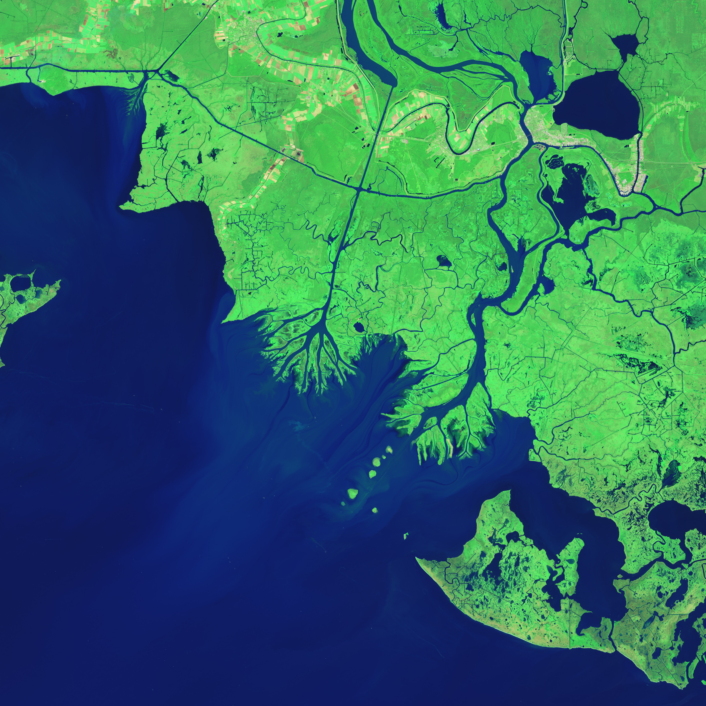
 1855 U.S. Coast Survey nautical chart or map of Tampa Bay, Florida.
Centered on Passage Point, this map covers from St. Helena and Tampa south to Mullet Key and Palm Key.
Chart notes various triangulation points and the proposed site of a rail depot on the western shore. The city of Tampa is noted though, at this stage, development is minimal.
Countless depth soundings fill the bay.
To the left of the map, below the title, are detailed sailing instructions and notes on tides and shoals. This is one of the earliest Coast Survey charts to focus on Tampa Bay. 
The hydrography for this map was completed by O. H. Berryman.
The chart was produced under the supervision of A. D. Bache, of the most prolific and influential Superintendents of the U.S. Coast Survey.
NOAA's Office of Coast Survey, based in Silver Spring, Md., was established in 1807 at the behest of President Thomas Jefferson, who wanted nautical maps drawn to improve shipping safety and to help the young nation's military better defend itself.
"Knowing more boats were destroyed by accident than war, they decided they needed to do a survey of the coast," Forsythe said.
"The first charts came out in the mid 1830s. We've been doing it ever since."

Maps were not produced every year – in the 1800s and well into the 1900s, it could take five to 10 years to produce a single map of a region.
It was a painstaking process.
Survey teams would measure water depths by dropping a lead ball attached to rope over the side of a ship until it hit bottom.
Then they would move about 500 feet and do it again, going back and forth, like a "mower over a lawn," Forsythe said.
Then engraved copper plates and a lithograph were used to produce a map.
Despite that tedious process, in the past 180 years, the Office Coast Survey has accumulated 35,000 historical maps of the entire U.S. coastline, covering about 3.4 million square miles.
"Now cartographers sit in front of computers," Forsythe said.
"About 150 charts are updated each week with critical corrections, available digitally."
While the maps are mainly used by the marine community, they also have been used by movie production companies to ensure accuracy of sets for given time eras.
And the behind-the-scenes data used to compile the maps has been used to develop storm surge prediction models, Forsythe said.
She added that the maps make great gifts for history and marine buffs.
"They are really cool to sit there and explore. It's another way of looking at history," she said.

Sunday, February 15, 2015

The Wedge : legendary backwash

Sunny morning in California by Alex Verharst

 
 Slow Motion Carnage

The Wedge with the Marine GeoGarage :
a surf break in Newport Beach CA that is known to be deadly.