The oceans are going to rise—but when?

The Thwaites ice shelf in West Antarctica is the floating extension of the Thwaites Glacier, which drains a large portion of the West Antarctic Ice Sheet.

The ice shelf is thinning due to melting by warm ocean water below.

From Quanta Magazine

The uniquely vulnerable West Antarctic Ice Sheet holds enough water to raise global sea levels by 5 meters.
But when that will happen—and how fast—is anything but settled.

In May 2014, NASA announced at a press conference that a portion of the West Antarctic Ice Sheet appeared to have reached a point of irreversible retreat.
Glaciers flowing toward the sea at the periphery of the 2-kilometer-thick sheet of ice were losing ice faster than snowfall could replenish them, causing their edges to recede inland.
With that, the question was no longer whether the West Antarctic Ice Sheet would disappear, but when.
When those glaciers go, sea levels will rise by more than a meter, inundating land currently inhabited by 230 million people.
And that would be just the first act before the collapse of the entire ice sheet, which could raise seas 5 meters and redraw the world’s coastlines.

At the time, scientists assumed that the loss of those glaciers would unfold over centuries.
But in 2016, a bombshell study in Nature concluded that crumbling ice cliffs could trigger a runaway process of retreat, dramatically hastening the timeline.
The Intergovernmental Panel on Climate Change (IPCC) took notice, establishing a sobering new worst-case scenario: By 2100, meltwater from Antarctica, Greenland, and mountain glaciers combined with the thermal expansion of seawater could raise global sea levels by over 2 meters.
And that would only be the beginning.
If greenhouse gas emissions continue unabated, seas would rise a staggering 15 meters by 2300.

However, not all scientists are convinced by the runaway scenario.
Thus, a tension has emerged over how long we have until West Antarctica’s huge glaciers vanish.
If their retreat unfolds over centuries, humanity may have time to adapt.
But if rapid destabilization begins in the coming decades through the controversial runaway process, the consequences could outpace our ability to respond.
Scientists warn that major population centers—New York City, New Orleans, Miami and Houston—may not be ready.

“We’ve definitely not ruled this out,” said Karen Alley, a glaciologist at the University of Manitoba whose research supports the possibility of the runaway process.
“But I’m not ready to say it’s going to happen soon.
I’m also not going to say it can’t happen, either.”

For millennia, humanity has flourished along the shore, unaware that we were living in a geological fluke—an unusual spell of low seas.
The oceans will return, but how soon? What does the science say about how ice sheets retreat, and therefore, about the future of our ports, our homes, and the billions who live near the coast?

Grounded by the Sea

In 1978, John Mercer, an eccentric glaciologist at Ohio State University who allegedly conducted fieldwork nude, was among the first to predict that global warming threatened the West Antarctic Ice Sheet.
He based his theory on the ice sheet’s uniquely precarious relationship with the sea.

Bigger than Alaska and Texas combined, West Antarctica is split from the eastern half of the continent by the Transantarctic Mountains, whose peaks are buried to their chins in ice.
Unlike in East Antarctica (and Greenland), where most ice rests on land high above the water, in West Antarctica the ice sheet has settled into a bowl-shaped depression deep below sea level, with seawater lapping at its edges.
This makes West Antarctica’s ice sheet the most vulnerable to collapse.

A heaping dome of ice, the ice sheet flows outward under its own weight through tentacle-like glaciers.
But the glaciers don’t stop at the shoreline; instead, colossal floating plates of ice hundreds of meters thick extend over the sea.
These “ice shelves” float like giant rafts, tethered by drag forces and contact with underwater rises and ridges.
They buttress the glaciers against an inexorable gravitational draw toward the sea.

ILLUSTRATION: MARK BELAN/QUANTA MAGAZINE

The critical frontline of the ice sheet’s vulnerability is the “grounding line,” where ice transitions from resting on the seafloor to floating as an ice shelf.
As the relatively warm sea works its way below the protective shelves, it thins them from below, shifting the grounding line inland.
The floating shelves fragment and break away.
The upstream glaciers, now without their buttressing support, flow faster toward the sea.
Meanwhile, seawater intrudes like an advancing army toward thicker ice, which rests on bedrock that slopes inward toward the bowl-like center of the continent.

“There’s a very serious message here,” said Hilmar Gudmundsson, a glaciologist at Northumbria University: As the grounding line marches inland toward ever-thicker ice in a process called marine ice sheet instability, “you will have a very sharp increase in global sea level, and it will happen very quickly.”

In 2002, scientists got a live view of how that process may play out.
The Larsen B ice shelf, a floating mass off the Antarctic Peninsula roughly the size of Rhode Island, broke apart in just over a month, stunning scientists.
Pooling surface meltwater had forced open cracks—a process called hydrofracturing—which splintered the shelf, the only barrier for the glaciers behind it.
The glaciers began flowing seaward up to eight times faster.
One of these, Crane Glacier, lost its cliff edge in a series of collapses over the course of 2003, causing it to shrink rapidly.
What if something similar happened to far larger glaciers on the coast of West Antarctica, like Thwaites and Pine Island?

In 2002, scientists watched with amazement as the Larsen B ice shelf collapsed in just over a month.
At the start of this series of NASA satellite images, pools of meltwater that contributed to the fracturing of the ice shelf are visible as parallel blue lines.
The shelf soon disintegrated into a blue-tinged mélange of slush and icebergs.
This ice debris field largely melted the following summer and began to drift away with the currents.
PHOTOGRAPH: NASA EARTH OBSERVATORY

In the years that followed, studies of ancient shorelines revealed a stunning sensitivity in the Earth system: It appeared that epochs only slightly warmer than today featured seas 6 to 9 meters above present-day levels.

In response, glaciologists Robert DeConto and David Pollard developed a bold new theory of ice sheet collapse.
They created a computer simulation based on Larsen B’s breakup and Greenland’s calving glaciers that was also calibrated to the geologic past—projecting future melt that matched expectations derived from ancient sea levels.

Their 2016 study outlined a scenario of almost unimaginably quick ice loss and sea-level rise.
In a process called marine ice cliff instability (MICI), cliffs taller than 90 meters at the edges of glaciers become unstable and collapse, exposing ever-thicker ice in a chain reaction that accelerates retreat.
The model suggested that ice from Antarctica alone—before any additions from Greenland, mountain glaciers or thermal expansion—could raise the seas by more than a meter by 2100.

In a 2021 update that incorporated additional factors into the simulations, DeConto and colleagues revised that estimate sharply downward, projecting less than 40 centimeters of sea-level rise by the century’s end under high-emission scenarios.
Yet even as the numbers have shifted, DeConto remains convinced of the MICI concept.
“It’s founded on super basic physical and glaciological principles that are pretty undeniable,” he said.

Mechanisms to Slow Retreat

After the 2016 study, the scientific community set out to test whether towering ice cliffs really could undergo runaway collapse.
Many soon found reasons for doubt.

Few dispute the basic physics: If ice shelves like Larsen B collapse quickly and expose tall-enough cliffs on the glaciers behind them, those cliffs will indeed buckle under their own weight.
“There’s a reason why skyscrapers are only so tall,” said Jeremy Bassis, a glaciologist and expert in fracture mechanics at the University of Michigan.
However, critics argue that runaway cliff collapse hasn’t been seen in nature, and there might be good reasons why not.

“Yes, ice breaks off if you expose tall cliffs, but you have two stabilizing factors,” said Mathieu Morlighem, a glaciologist at Dartmouth College who led a 2024 study that identified these factors.
First, as newly exposed glacier cliffs topple, the ice behind stretches and thins.
As this happens, rapidly, “your ice cliff is going to be less of a tall cliff,” Morlighem said.
Second, the flowing glacier brings more ice forward to replace what breaks off, slowing the cliff’s inland retreat and making a chain reaction of cliff toppling less likely.

Another study challenging the MICI scenario noted that breaking ice also tends to form a mélange, a dense, jumbled slurry of icebergs and sea ice.
This frozen slurry can act as a retaining wall, at least temporarily stabilizing the cliffs against collapse.

The bedrock beneath the ice might also be a key player.
“The solid Earth is having much bigger impacts on our understanding of sea-level change than we ever expected,” said Frederick Richards, a geodynamicist at Imperial College London.
Scientists have long recognized that when glaciers melt, the land rebounds like a mattress relieved of weight.
But this rebound has been mostly dismissed as too sluggish to matter for several centuries.
Now, high-precision GPS and other geophysical data reveal rebound occurring over decades, even years.

Whether that’s good or bad depends on how quickly ice retreats.
If it goes at a modest clip, the bedrock lifts the ice, reducing the amount of water that can lap away at it.
But if retreat happens quickly enough through something like runaway cliff collapse, the Earth can’t keep up.
A 2024 study showed that the bedrock still rises, but in that scenario it pushes meltwater into the ocean.
“You’re actually getting more sea-level rise,” Richards said.
“You’re pushing all this water out of a bowl underneath West Antarctica and into the global ocean system.”

Earth’s restlessness also affects models of ancient sea-level rise.
In a 2023 study, Richards and colleagues found that Australia’s 3-million-year-old Pliocene shorelines had ridden the slow heave and sigh of Earth’s mantle, and that accounting for that vertical motion resulted in lower estimates for ancient sea levels.
This matters, according to Richards, because the revised record is a better match for more conservative ice retreat models.
“Hold on, guys,” he said.
“We have to be a little bit careful.
[Ancient] sea-level estimates might be overestimates, and therefore we might be overestimating how sensitive the ice sheets are.”

DeConto points to the Larsen B breakup and the crumbling of Greenland’s Jakobshavn Glacier as evidence to the contrary.
Once Larsen B stopped holding back the Crane Glacier, he says, ice began breaking away faster than the glacier could replenish it.
That is “really strong evidence that fracture can outpace flow.”
From Past to Future

“When I started my career, the question was whether Antarctica was growing or shrinking,” said Ted Scambos, a glaciologist at the University of Colorado, Boulder.
The IPCC long held that the ice sheet would remain relatively stable through the 21st century, on the logic that rising temperatures would bring more snow, offsetting melt.

That assumption collapsed along with Larsen B in the early 2000s, and scientists soon came to a consensus that ice loss was well underway.
Satellite observations revealed that glaciers along the Amundsen Sea, including Pine Island and Thwaites, were flowing faster than in previous decades.
The ice sheet was not in balance.
By the time NASA called the 2014 press conference, it was clear that many of West Antarctica’s enormous glaciers had been retreating steadily since the 1990s.

The aftermath of Hurricane Florence in Myrtle Beach, South Carolina in 2018.
Worldwide, some 230 million people live less than a meter above sea level, and 1 billion people are within 10 meters of sea level.
CREDIT: NATIONAL GUARD/ALAMY

“It was the first time we had enough observations to say, hey, look, these grounding lines have been retreating year after year,” said Morlighem, a coauthor on one of the studies presented at the press conference.
This steady loss signaled that the glaciers would inevitably disappear.
“In theory, if we turn off melt, we can stop it,” he noted.
“But there’s absolutely zero chance we can do that.”

While the conversation has centered on how the sea will lap away at the ice shelves, some scientists are increasingly concerned about what’s happening up top, as warming air melts the ice sheet’s surface.
Nicholas Golledge, a glaciologist at Victoria University of Wellington, sees West Antarctica today as transitioning to the status of Greenland: Most of Greenland’s marine-vulnerable ice has already vanished, and surface melt dominates.
That process, Golledge believes, may soon play a bigger role in Antarctica than most models assume.

Pooling meltwater, for example, contributed to the Larsen B collapse.
As the water trickles into crevasses, it lubricates the bedrock and sediments below, making everything more slippery.
The Columbia University glaciologist Jonny Kingslake says these processes are oversimplified or omitted in numerical simulations.
“If you ignore hydrology change, you are underestimating retreat,” he said.

Indeed, a 2020 study found that meltwater trickling into Antarctica’s ice shelves could infiltrate cracks and force them open, a precursor to marine ice cliff instability that DeConto and colleagues envisioned.

Depending on future emissions, the IPCC now projects an average sea-level rise of half a meter to 1 meter by 2100, a total that includes all melt sources and the expansion of warming water.
The MICI process, if correct, could accelerate Antarctica’s contribution enough to double that overall rise.
“There’s deep uncertainty around some of these processes,” said Robert Kopp, a climate scientist and science policy expert at Rutgers University.
“The one thing we do know is that the more carbon dioxide we put into the atmosphere, the greater the risk.”

In Bassis’ view, “Whether it’s with marine ice cliff instability or marine ice sheet instability, it’s a bit of a distraction.
By 2100, we will be talking about a coastline radically different than what I grew up with.”

Shipping companies call for better Arctic navigation tech as trips get tougher

 

From The Canadia Press by Christopher Reynolds
 

Shipping companies are calling on the federal government to invest in Arctic infrastructure and navigation technology as climate change renders transport corridors more hazardous — even as traffic ramps up.

Northern waters need new port facilities, higher quality satellite imaging and modern mapping that charts the depth of the ocean floor, say a group of more than a dozen ship owners and transport companies.

"There's a growing need for transportation in the Arctic," said David Rivest, president of Desgagnés Transarctik, a shipping firm that supplies dozens of northern communities.

Infrastructure upgrades would help meet the expanding needs of northern communities and mining firms as well as the threat of foreign actors amid rising global tensions, according to the St.
Lawrence Ship Operators association.

Longer, sturdier boat ramps are one example.

"These ramps are essentially just gravel inclinations going from the water up to a beach landing area," Rivest said.
"They're exposed to the tides."

In communities where food, building materials and consumer items come primarily by ship, transport tugs can haul barges up to the ramp at high tide.
But at low tide, shallow water and rocks make landing tricky or impossible.

A new landing zone — in a nearby bay with better boat access and shelter from wind and storms, for example — would make the process much more efficient, Rivest said.

"For instance, in Kuujjuaq, a very important community in northern Quebec, we have to anchor four or five nautical miles away from the ramp. That means there's a long transit between the ship and the beach area," he said.

Efficiency is all the more crucial in areas with short seasonal windows for seaborne deliveries.
The Arctic shipping season typically runs from June through November.

"But there's certain locations where we can only deliver 45 days," Rivest said.
"Sometimes it's even less than that."

Meanwhile, a retreat in Arctic sea ice has opened up waterways to more boats, making passage more treacherous, but also unleashed icebergs that can hamper ships.

"Early this summer, we had a ship that was out west in the Northwest Passage, and I was completely surprised to find dozens of sailboats crossing west to east, meeting our ships in the area," said Daniel Dagenais, CEO of NEAS Group, which hauls everything from diesel tanks to roof trusses to towns and villages across the North.

The number of boat trips into Canadian Arctic waters increased by nearly half to 466 between 2011 and 2024, a study out of the Université du Québec à Montréal found.

Shippers say that steady increase in both traffic and ice flows demands better navigation tech — weather tracking systems and satellite image processing, for example.

As of May 2023, 15.8 per cent of Canadian Arctic waters had been "adequately surveyed," while 44.7 per cent of its key navigational routes met that standard, according to the Canadian Hydrographic Service.

Oceans and Thermometric Gateways to the North Pole - 1872 map 

by US Navy hydrographer Silas Bent. 

In the 1800s many geographers mistakenly believed the Arctic was an open ocean 

surrounded by a ring of ice.

 
"With the warming temperatures, it's a lot more volatile," Rivest said of ice flows.
"It's moving around, it's going into these main transit areas and then the ships need to take alternate courses.
"Compound that with the bathymetry" — topography mapping, but for water bodies — "that's not up to date, you accentuate the risks for incidents," he said.
"Think of going on Google Maps today and trying to look at the map of Canada and 85 per cent of it is not there. That's what we're dealing with when we're navigating in the Arctic."

The shipping association has welcomed Ottawa's renewed focus on infrastructure projects and defence spending, which could have northern applications ranging from radar stations to housing.
But precisely how the dollars in the recent federal budget will find their way to Arctic shipping remains uncertain.

"It all trickles down in the weeks and months that come afterwards, so that's where we need more details," said association executive director Saul Polo.

As Prime Minister Mark Carney seeks to make sovereignty a central theme in his government, shippers hope to shine a light on the defence benefits of broader federal investment in the North.

 

On top of surveillance and mapping gear, infrastructure ranging from housing and research stations to coast guard icebreakers and search-and-rescue crews could serve both commercial and military goals, the association argues.

"There's more and more demands in the Arctic, and it's not about to go away," Dagenais said.

 

Links :

• The Economist : The Arctic will become more connected to the global economy 
• NOAA : Arctic Report Card: Update for 2025 

France & misc. (SHOM) layer update in the GeoGarage platform

 

2 new raster charts added & 239 charts updated

see GeoGarage news 

 

Was Hvaldimir the whale really trained by the Russian military?

Hvaldimir has been suspected of espionage for Russia since 2019. (Photo: Marine Mind)

 

From ScienceNorway by Annbjørg Hjelmevoll

 

Since the Cold War, the Soviet Union and the USA have trained belugas and dolphins to defend bases and submarines.

Hvaldimir might have been one of them before he escaped. 

One day in 2019, the beluga whale Hvaldimir was discovered near Ingøy in northern Norway. It had a camera harness on and was very sociable, according to the Norwegian Broadcasting Corporation NRK.

The whale stayed in the Hammerfest area for a long time before starting to move up and down the Norwegian coast.

Hvaldimir was both in the Oslofjord and in Fjällbacka in Sweden before being found dead in Risavika in sourthern Norway in 2024.

In a BBC documentary, Ukrainian marine biologist Olga Shpak stated that the beluga Hvaldimir is believed to have escaped from a Russian military programme.
She has researched whales in Russia since the 1990s before returning to Ukraine in 2022.
She said her Russian colleagues told her that the navy immediately identified Hvaldimir as one of their own.

In Russia, the whale was named Andruha. 
When the trainers started working with the beluga in open water, Hvaldimir reportedly swam away from the boat he was supposed to follow, Shpak told the BBC.
Audun Rikardsen, a whale researcher at UiT The Arctic University of Norway, told sciencenorway.no that he was always certain Hvaldimir came from the Russian navy.
Russia has never responded to whether Hvaldimir was trained by them, but the use of belugas in defence is nothing new.

The 'Dolphin Arms Race'

Since the 1960s, both the USA and the former Soviet Union have used belugas, dolphins, and sea lions to protect naval bases, according to The Guardian. 
It was the Americans who began training marine mammals for defence.

This became part of the major arms race with the Soviet Union during the Cold War.

This image from 2003 shows an American military dolphin

(Photo: AP Photo / Petty Officer First Class Brien Aho)

According to Rikardsen, belugas are used in colder, northern areas, while dolphins and sea lions are more common in warmer regions.
Russia is also said to have used dolphins to protect the Black Sea fleet's base from Ukrainian attacks in Sevastopol on the Crimean Peninsula during the war, writes The Guardian.

Why train belugas and dolphins?

One of the traits that make belugas and dolphins attractive to the military is their use of echolocation. This means they use sound to navigate underwater.
As a result, they are not as dependent on vision as humans are, marine biologist Sebastian Strand at Marine Mind explains.

Marine mammals are not hindered by darkness, making it easier for them to perform certain tasks. 
Moreover, they can swim faster and dive deeper than humans without getting sick. 
They are used to search for underwater mines, sabotage divers, and submarines.
According to Strand, belugas are trained to attach magnets to diving tanks, with a rope and buoy hanging from it. The buoy floats to the surface of the water.
"It gives a 'There's a person here!' signal," he says.
Marine mammals can also be tasked with sabotaging enemy boats. Strand explains that this can be done by attaching objects to boat propellers to disable them. 

Satellite images from Goryarchiye Ruchyi in Kolabukta near Murmansk, Russia.

The image shows the beluga facility Hvaldimir may have belonged to before he escaped.

(Photo: Annbjørg Hjelmevoll / Google Earth)

According to Russian military expert Viktor Baranets, dolphins were also trained to survey the seabed, defend marine areas, and attach explosives to the hulls of ships, writes NRK.

Hvaldimir as a military whale

"We saw clear signs of training. There was no doubt about it," says Strand. 
Strand explains that he saw Hvaldimir doing things consistent with tasks military whales are trained for. 
He personally monitored the whale for three years and became well-acquainted with Hvaldimir's patterns.

Strand worked as an advocate to protect the whale from human interference.

Firstly, Hvaldimir was very eager to retrieve objects from the sea.
You may have seen the video of the beluga rescuing a girl's phone when she dropped it in the water in Hammerfest? 
Secondly, it seemed like Hvaldimir enjoyed attaching loose ropes to boat propellers. 

Hvaldimir plays with a rope near a fish farm in Sørfolda. (Photo: Audun Rikardsen)

This became a small issue for those working with salmon farming, and Strand explains that he often had to step in to help untangle the rope from the boats. 
Strand mentions that they had to be careful not to create a connection between attaching the rope and their appearance.
"Hvaldimir was really clever and wanted to see the people he became familiar with again," he says.

To ensure it wasn't a reward for the whale when they showed up, Strand had to wait until Hvaldimir left the area before fixing the propeller.
Rikardsen thinks there could be several reasons why Hvaldimir enjoyed being near fish farms. There was plenty of food in the area, and the facility might have resembled his childhood home in Russia.
"We can never fully confirm what he was actually trained for. This is speculation based on Hvaldimir's behaviour," says Rikardsen.

Like humans, Hvaldimir had a taste for fast food.

(Photo: Antoine Drancey / Marine Mind)

"But no one has seriously thought that Hvaldimir was sent across the border to spy. That was said as a joke in the beginning,” he adds.

Similar to guard dogs

Many may find it strange that whales can be trained to carry out such tasks. 
However, Strand says the traits sought in animals for training aren't so different from when wolves were domesticated into what we now know as dogs.
"We think of dogs as cooperative, and this sounds crazier when it comes to marine mammals. But when we hear about guard dogs alerting us to intruders, that seems natural," he says.

Hvaldimir was always happy to greet people. (Photo: Marine Mind)

Belugas are intelligent and social herd animals that naturally communicate and cooperate extensively with others. This makes them easier targets for training.

"They have cooperation coded into their behaviour," says Strand.

Hvaldimir's death

Hvaldimir was found dead in August off the coast of Risavika southern Norway with multiple injuries on his body.
Investigations conducted by the Norwegian Veterinary Institute and police forensic experts indicate that Hvaldimir likely died from a bacterial infection caused by a wound in his mouth, according to NRK.

 

Links :

• BBC : Russian 'spy whale' was not shot, say police
• The Guardian : New film unravels mystery of the Russian ‘spy whale’ 

Satellite imagery for hazard detection: better use of satellite imagery could help prevent groundings in the Canadian Arctic

On September 6th, the MV Thamesborg, a Dutch cargo ship enroute from China to Quebec, Canada, ran aground in the Canadian Arctic.

Its draught is up to ~9.4 meters, and it ran aground on a shoal charted as 20.2 meters deep!

In my research I detect shallow water from satellite imagery, and my results suggest that the shallowest section of this shoal is ~8.9 meters deep (there's uncertainty around that number!).

This particular shoal is also directly visible in satellite imagery - one just needs to look carefully.

From IHO by Anders Knudby

Abstract

This study demonstrates how satellite imagery can reduce the risk of grounding in poorly surveyed waters.
Automated shoal detection and satellite-derived bathymetry (SDB) were applied to Sentinel-2 imagery for seven grounding sites in the Canadian Arctic.
Shoal detection was successful for all sites, and SDB showed depths as shallow as 0.3 m.
Proactive use of satellite imagery, even without advanced image processing, could have provided mariners with vital information on the location of uncharted shoals and prevented costly and dangerous accidents.
The hydrographic community should accelerate the inclusion of satellite-derived products into the information provided to mariners for safety of navigation.

1 Introduction

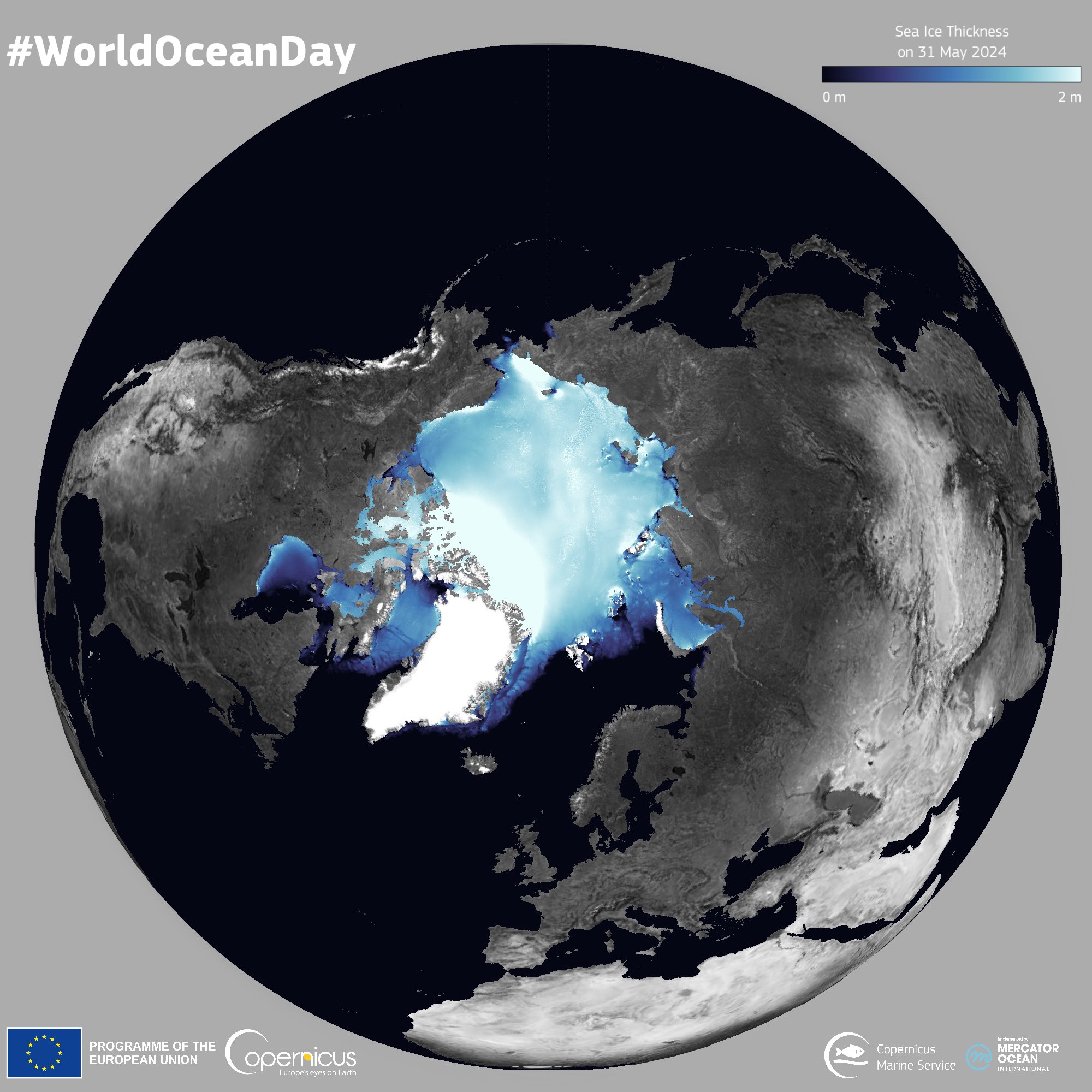
The Arctic Ocean is experiencing profound and rapid climatic changes, with significant implications for sea ice, navigability and maritime transportation.
Human-induced warming has accelerated the decline in sea ice extent and thickness (Yadav et al., 2020), lengthening the ice-free season, and projections suggest that the Arctic could experience nearly ice-free summers as early as 2030 (Kim et al., 2023).
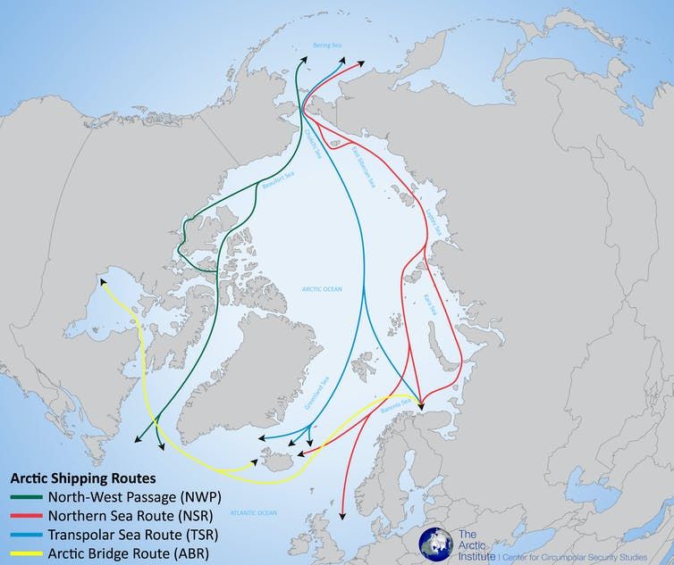
These changes allow the opening of new shipping routes into and across the Canadian Arctic, routes that are becoming more accessible for longer periods each year (Liu et al., 2024).
Recent years have seen an increase in maritime transportation in the Canadian Arctic Ocean (Dawson et al., 2018).
In 2024, 466 ship voyages were recorded in Canadian Arctic waters, compared to 301 in 2014, a 55 % increase over the last decade, despite excluding data from November and December 2024 (Lasserre & Baudu, 2024).

However, the Canadian Arctic Ocean remains poorly surveyed and charted.
The Canadian Hydrographic Service (CHS) estimates that only 15.8 % of Canadian Arctic waters have been adequately surveyed, including only 44.7 % of key navigational routes, and many charts contain minimal or insufficient information to support safe and efficient navigation (CHS, 2023).
Many areas outside shipping corridors contain only outdated survey data, or no data at all, leading charts to be sparsely populated with soundings or simply contain white space with no information.
The soundings that do exist can be over 100 years old, created from lead line measurements with positioning based on triangulation to points on land, the locations of which are themselves of unknown accuracy (Government of Canada, 2014).
Even the distinction between land and water is sometimes incorrect on older CHS charts.
For example, while supporting recent updates to CHS charts 7185 and 7193, the author identified the correct location of an island charted almost 2 km from its actual location, in addition to numerous previously uncharted shoals.
An island >500 m across, which had been charted as a shoal, was also identified (Fig. 1).
Such incomplete and erroneous charts, combined with increasing production and mobility of icebergs in the Arctic Ocean (Dalton, 2023) and increasing maritime traffic, inevitably create a substantial risk to the safety of navigation in Canada’s Arctic (Howell et al., 2024; Nicoll et al., 2024; TSB, 2010).

Fig. 1 During work to update CHS chart 7185, a shoal indicated in the chart from 2016 (A) was found in satellite imagery to be an island larger than 500 m across (B), allowing it to be positioned and outlined correctly in the updated chart (C).

While groundings are relatively infrequent in the Canadian Arctic due to the small total number of voyages, compared to other marine regions the Arctic has the highest accident rate at ~10 accidents per 1000 commercial ship movements (Council of Canadian Academies, 2016).
Approximately 16 % of these are groundings (TSB, 2025).
From 2000 to 2018, the Transportation Safety Board of Canada (TSB) received reports of 74 instances of vessel grounding or bottom contact in the Canadian Arctic.
The severity of these occurrences varies; some vessels sustain little to no damage and simply refloat at high tide, while others result in hull damage and breached fuel tanks, pollution, evacuation of crew and passengers, and high costs for search and rescue, cleanup, and repairs (TSB, 2021).
A substantial number of these groundings occur on uncharted shoals; some of these shoals are known to the CHS but not included on charts and instead communicated to mariners through the use of Notices to Shipping (NOTSHIP; TSB, 2010).
Others only become known after a grounding has occurred.

Satellite imagery remains underutilized in Canada’s Arctic, especially for identifying hazards not included on official charts.
While most shoals are not known to CHS in advance of a vessel grounding, many of them are nonetheless easily detectable using satellite imagery.
Water is typically clear throughout much of the Arctic Ocean and shoals are often easily visible in optical satellite imagery.
This includes free and publicly available imagery such as that provided by the Sentinel-2 MultiSpectral Instrument (MSI), for which imagery has been available for most of the Arctic Ocean since 2015 (Trémas et al., 2015).
These shoals can be identified either using automated image processing algorithms (Richardson et al., 2024) or simply by visually inspecting the imagery and delineating the areas where the seafloor is visible.
In areas of high turbidity, as is typical in glacial fjords or near river outlets, or under other unsuitable environmental conditions (e.g.
in the presence of ice cover, cloud shadowing, whitecaps, or excessive sunglint), detection and delineation of shoals from optical satellite imagery is not always possible.
But for large parts of the Arctic Ocean shoals are clearly visible to depths of at least ~10 m.

In addition to delineation of the locations and extents of shoals, a variety of algorithms exist to estimate the depth of water from the colour of the area as observed in a satellite image.
These algorithms are collectively known as satellite-derived bathymetry (SDB) and can be used to approximate the depth of shoals.
Most SDB algorithms employ one of two approaches.
In empirical SDB, trusted geolocated water depth measurements, typically obtained with acoustic or lidar instruments, are used to establish an empirical relationship between pixel colour and water depth.
That relationship is then extrapolated to the parts of the image for which water depths are to be estimated (Caballero & Stumpf, 2023; Ilori et al., 2019; Knudby & Richardson, 2023; Lyzenga, 1985, 1978; Stumpf et al., 2003).
An alternative approach, often termed physics-based SDB, inverts a radiative transfer model by matching the color observed in each pixel to a set of realistic environmental parameters, including water depth, that it most closely matches (Dekker et al., 2011; Hedley et al., 2012; Knudby et al., 2016; Lee et al., 1999).
This approach eliminates the need for trusted geolocated water depths measurements, which often do not exist in the Canadian Arctic, but instead relies on the ability to accurately account for all environmental factors that influence how water depth influences pixel color.
Less-used alternative approaches to SDB also exist, including the use of photogrammetry (Hodúl et al., 2020, 2018) and wave-based kinematics (Daly et al., 2022).
SDB is increasingly used in production of nautical charts, including by the United Kingdom, France, the United States (Mavraeidopoulos et al., 2017), and more recently Canada (Ahola et al., 2020; Chénier et al., 2018).
However, despite the availability of satellite imagery for the entire Canadian Arctic, operational application of SDB has been limited.

The limited bathymetric information displayed on many charts of the Canadian Arctic, contrasted with the wealth of such information available in satellite imagery, suggests that an expanded use of satellite imagery for providing bathymetric information to mariners would be beneficial and could help reduce the frequency of groundings in Canada’s increasingly busy Arctic Ocean.
In this study, satellite imagery is used for i) shoal detection and ii) SDB, to illustrate the potential for satellite imagery to provide information that could reduce the risk of navigation in poorly charted waters.
The study is based on seven cases from the Canadian Arctic Ocean, each featuring a vessel grounding on a shoal that a) is clearly visible in satellite imagery but b) was uncharted at the time of grounding.

2 Data and methods

2.1 Groundings

Relevant case studies were identified using the TSB’s publicly available marine transportation occurrences database (TSB, 2025).
As of February 2025, the database contained 86124 occurrences from 1975 to 2025 (many entries were duplicates, so the actual number of occurrences is smaller).
Occurrences were first filtered to include only those classified as bottom contact or grounding under power, outside a harbor area, and located north of 65 °N, leaving 760 occurrences.
Of those, seven were chosen for inclusion in this study based on i) their location in the Canadian Arctic Ocean, ii) the visibility of shoals in satellite imagery, iii) a desire to achieve a geographically distributed set of cases, and iv) other factors, such as weather, that indicate that the groundings could have been avoided if the shoals had been included on CHS charts, and v) the need to focus on a subset of occurrences for investigation.
The resulting set of selected groundings is outlined in Table 1 and shown on Fig.
2.
As per the criteria listed above, this is not intended to be an exhaustive or representative list of groundings in the Canadian Arctic Ocean.
Interested readers are referred to the TSB’s official list of occurrences for more examples.

2.2 Satellite imagery and CHS charts

For each grounding site, all Sentinel-2 images available from July to October for the years 2023 and 2024 were accessed, imagery with >50 % cloud cover was removed, and the remaining images were visually assessed to remove those with substantial ice cover, haze, or other environmental conditions rendering them unsuitable for SDB.
As a result, between nine and thirteen images were available for each grounding site.
The location, date and year of each grounding was used to identify the CHS chart that was current, i.e.
the chart that the vessel crew would have had access to, at the time of grounding.
These charts were located and accessed from Libraries and Archives Canada and scanned on a large-format scanner.
A section of the relevant chart surrounding each grounding site was then manually georeferenced based on distinctive coastline features, using the Sentinel-2 satellite imagery for reference.

2.3 Shoal detection

For shoal detection, a global model for delineation of optically shallow water (Richardson et al., 2024) was applied to the Sentinel-2 images available for each site.
For each image, this model produces a per-pixel probability of water being optically shallow, i.e.
the probability that the seafloor is visually detectable in the imagery, after applying a mask to exclude non-water pixels.
To identify shoals, the mean unmasked value of these per-image probabilities was then calculated, and pixels with a resulting value greater than 50 % were labeled as shoals.
Visual examination of the results suggested that this 50 % threshold achieved a good trade-off between limiting false positives (image noise labeled as shoals) and limiting false negatives (undetected shoals).

Table 1 List of the seven groundings included in this study, in chronological order.

 

Fig. 2 The locations of the seven groundings used in this study, within the Canadian Arctic Archipelago.

2.4 Satellite-derived bathymetry

For SDB production, the Fully Automated Bathymetry (FAB) workflow, developed by Liquid Geomatics Ltd. was employed.
FAB processing is based on 100 km × 100 km Sentinel-2 image tiles; products for smaller areas such as those surrounding each of the grounding sites illustrated in this paper can be extracted from the larger tiles.
FAB processes Sentinel-2A and -2B images end-to-end, including image download from Copernicus Dataspace, land and cloud masking, deglinting (optional), atmospheric correction (Hedley, 2018), bathymetry estimation based on radiative transfer model (RTM) inversion (Hedley et al., 2009), correction for tide level at image acquisition (Lyard et al., 2021), and ensemble predictions based on multiple images for each site (Ilori & Knudby, 2020).
FAB is implemented in Python 3.11, with calls to the IDA software (Hedley, 2019) for deglinting, atmospheric correction and RTM inversion (Hedley et al. 2018; Casal et al., 2020).
Detailed information on data processing in the FAB workflow is provided in Appendix A.

2.5 SDB accuracy assessment

For most of the grounding sites, no or insufficient acoustic data was available to assess the accuracy of the SDB bathymetry maps produced with FAB.
For the two sites where data was available, namely the grounding sites of the Clipper Adventurer and V/L Camsell, NONNA10 data was downloaded from CHS (CHS, 2024) and reprojected to match the spatial reference system of the relevant Sentinel-2 imagery.
Sentinel-2 imagery is distributed projected to WGS-based UTM zones based on the Military Grid Reference System (MGRS).
CHS’s NONNA data is a set of non-navigational bathymetric survey data, compiled from individual surveys and made publicly available in raster format.
For the Clipper Adventurer site, most of the NONNA data came from a 2010 multi-beam survey conducted following the grounding.
This survey covered the entire shoal and the immediate surroundings and is categorized as Zone of Confidence (CATZOC) A2.
For the V/L Camsell site, ~95 % of the NONNA data came from an Airborne Lidar Bathymetry (ALB) survey from 1986 categorized as CATZOC B; a few additional data points came from a single-beam survey conducted sometime between 1955 and 1964, categorized as CATZOC C.
Bathymetry was extracted from overlapping SDB and NONNA10 pixels for comparison and calculation of the coefficient of determination (R2) and the mean absolute difference (MAD) between the two data sets.
This comparison was limited to SDB depths <= 10 m, beyond which the accuracy of SDB estimates in this region rapidly degrades due to the decreasing magnitude of the bottom-reflected optical signal recorded in the satellite imagery.

3 Results

3.1 The groundings

Below, a review of i) the CHS chart at the time of grounding, ii) satellite imagery of the grounding site, and iii) the shoal detection and FAB SDB products, is provided for the most recent four groundings listed in Table 1.
Similar reviews for the remaining three groundings are provided in Appendix B.

3.1.1 Clipper Adventurer grounding

On 27 August 2010, the Clipper Adventurer ran aground on a known but uncharted shoal in Coronation Gulf, Nunavut, during calm seas and with clear visibility.
All passengers were uninjured but evacuated from the vessel, and minor pollution was reported.
The vessel was successfully refloated after multiple attempts conducted over a ~2-week period (TSB, 2010).
Fig. 3 shows a comparison between the relevant subset of the 1990 version of CHS chart 7777, current at the time of the grounding (A), satellite imagery of the area (B, C), the shoal detection product (D), and the FAB SDB product (E).
Soundings on the chart appear in a single line passing closely to the northeast of the shoal on which the Clipper Adventurer grounded.
The shoal is clearly visible in the satellite imagery, identified in the shoal detection product, and the FAB SDB product indicates that it has a minimum depth of 4.0 m.
For comparison, the draught of the Clipper Adventurer is 4.5 m (forward) and 4.6 m (aft) (TSB, 2010), making prior knowledge of a shoal at 4.0 m depth critically important to navigational decision-making.
This particular shoal had actually already been reported in 2007 by the Canadian Coast Guard Ship (CCGS) Sir Wilfrid Laurier, leading to the publication of a Notice to Shipping (NOTSHIP) that indicated a minimum depth of 3.3 m.
However, CHS determined that the information provided from Sir Wilfrid Laurier did not meet the requirements for a permanent chart update and instead planned a detailed survey for 2009 to produce data of sufficient quality.
Ultimately this did not happen until after the Clipper Adventurer grounding in 2010.
In the meantime, in 2008, another passenger vessel, the Akademik Ioffe, passed near the same shoal.
The crews of both vessels were unaware of the NOTSHIP that reported the shoal’s existence (TSB, 2010).

 

Fig.
3 Comparison of a subset of CHS chart 7777 from 1990, current at the time of grounding (A), a Sentinel-2 satellite image covering the same area (B), a section of the satellite image showing the shoal on which the grounding happened in greater detail (C), the same satellite image with the shoal detection product overlaid (D), and the same satellite image with the FAB SDB product overlaid (E).
The extent of the areas shown in (C-E) is indicated by the red rectangles in (A) and (B).
Note that the location of the grounding reported by TSB is approximately 500 m SE of the shoal shown here, which was correctly identified on the basis of the CHS survey that followed the grounding.

3.1.2 Akademik Ioffe grounding

On 24 August 2018, the passenger vessel Akademik Ioffe ran aground 78 nautical miles north-northwest of Kugaaruk, Nunavut, in an area almost entirely without charted bathymetric information.
The vessel was refloated the same night, and the passengers, all uninjured, were evacuated the next morning.
Minor pollution was reported (TSB, 2021).
Fig. 4 shows a comparison between the relevant subset of the 1998 version of CHS chart 7502, current at the time of the grounding (A), satellite imagery of the area (B, C), the shoal detection product (D), and the FAB SDB product (E).
Two soundings appear on the subset of the chart shown in Fig.
4, indicating depths of 71 and 92 meters respectively, both over 2 km from the shoal on which the Akademik Ioffe ran aground.
This corresponds to the note on the chart that the charted information is “of a reconnaissance nature collected from CHS spot sounding surveys”.
The shoal appears faint but is clearly visible in the satellite image, correctly detected by the shoal product, and the FAB SDB product indicates a minimum depth of 4.5 m.
The draught of the Akademik Ioffe is 5.9 m

 

. 

Fig. 4 Comparison of a subset of CHS chart 7502 from 1998, current at the time of grounding (A), a Sentinel-2 satellite image covering the same area (B), a section of the satellite image showing the shoal on which the grounding happened in greater detail (C), the same satellite image with the shoal detection product overlaid (D), and the same satellite image with the FAB SDB product overlaid (E).
The extent of the areas shown in (C-E) is indicated by the red rectangles in (A) and (B).

3.1.3 Hanse Explorer grounding

On 23 August 2019, the yacht Hanse Explorer ran aground in Admiralty Inlet, Nunavut.
No pollution or injuries were reported, and the vessel sustained only minor damage.
Approaching Levasseur Inlet, “the under-keel water depth abruptly diminished from 44 m to 0 m and the vessel ran aground” (TSB, 2021).
Fig. 5 shows a comparison between the relevant subset of the 1985 version of CHS chart 7568, current at the time of the grounding (A), satellite imagery of the area (B, C), the shoal detection product (D), and the FAB SDB product (E).
No soundings are charted in or near Levasseur Inlet; a single line of soundings are charted for Admiralty Inlet (west of the area shown in Fig. 5).
A shoal dominating the entrance to Levasseur Inlet is clearly visible in the satellite imagery (C), and is correctly detected by the shoal product, though with central parts of the shoal missing (not indicated as shoal).
FAB SDM estimates a minimum depth of 0.3 m for the part of the shoal where the grounding occurred.
The draught of the Hanse Explorer is 4.3 m.

 

. 

Fig. 5 Comparison of a subset of CHS chart 7568 from 1985, current at the time of grounding (A), a Sentinel-2 satellite image covering the same area (B), a section of the satellite image showing the shoal on which the grounding happened in greater detail (C), the same satellite image with the shoal detection product overlaid (D), and the same satellite image with the FAB SDB product overlaid (E).
The extent of the areas shown in (C-E) is indicated by the red rectangles in (A) and (B).

3.1.4 Martin Bergmann grounding

On 03 September 2014, the Martin Bergmann ran aground in largely uncharted waters near Gjoa Haven, eastern Queen Maud Gulf, Nunavut, while searching for Sir John Franklin’s lost ships, HMS Erebus and HMS Terror.
Weather conditions during the grounding were not reported.
Fig. 6 shows that the chart contains two soundings just west of the shoal that caused the grounding, but very sparse bathymetric data are charted in the area near the grounding, which contains many shoals.
The shoal that caused the grounding is clearly visible in the satellite image, correctly detected in the shoal product, and the FAB SDB indicates its minimum depth as 0.3 m.
With a draught of 3.43 m (Arctic Focus, 2025), knowledge of this shoal and its minimum depth would have had obvious implications for navigation of the Martin Bergmann.

 

 

Fig. 6 Comparison of a subset of CHS chart 7083 from 1980, current at the time of grounding (A), a Sentinel-2 satellite image covering the same area (B), a section of the satellite image showing the shoal on which the grounding happened in greater detail (C), the same satellite image with the shoal detection product overlaid (D), and the same satellite image with the FAB SDB product overlaid (E).
The extent of the areas shown in (C-E) is indicated by the red rectangles in (A) and (B).

 

3.2 SDB accuracy

Comparison between the FAB SDB estimates and survey data provided by CHS in the form of NONNA10 rasters was limited to depths up to 10 m due to the rapid degradation of SDB performance at deeper depths.
This comparison, possible only for the shoals on which the Clipper Adventurer and V/L Camsell ran aground due to the limited coverage of CHS data, shows that FAB SDB performs similarly to what is reported for SDB products elsewhere in the Arctic (Ahola et al., 2020; Chénier et al., 2018).
The comparison for the Clipper Adventurer (Fig. 7A; n = 380, R2 = 0.58), shows a slight bias toward depth overestimation, with depths overestimated by an average of 0.71 m, and a mean absolute difference between SDB and survey data of 1.04 m.
The comparison for V/L Camsell (Fig. 7B; n = 78, R2 = 0.45) instead shows a slight bias toward depth underestimation, with depths underestimated by an average of 0.89 m, and a mean absolute difference between SDB and survey data of 1.35 m.
Given these error statistics, the FAB SDB product would not meet International Hydrographic Organization (IHO) Order 2 specifications for vertical accuracy and would be categorized as CATZOC D data.
In consequence, and as has been the practice at CHS, the FAB SDB product should not be directly used for charting.
However, it is important to note that especially the comparison of FAB SDB to the CATZOC B and C survey data available for the V/L Camsell grounding site, and the resulting error statistics, should be interpreted considering the quality of the CHS data available for that comparison.
It is possible that the relatively lower R2 and larger MAD of the FAB SDB product at the V/L Camsell grounding site is due to the lower quality of the data used for comparison at this site.

 

Fig.
7 Scatter plots comparing bathymetry estimates from FAB SDB (y-axes) to NONNA10 bathymetry data from CHS (x-axes) for the two groundings sites for which data were available: the site of the Clipper Adventurer (A) and V/L Camsell (B).

4 Discussion

This study presented a review of seven groundings that occurred on shoals in the Canadian Arctic.
All these shoals are clearly visible and easily detectable in satellite imagery but were not indicated on the CHS charts current at the time of each grounding.
SDB applied to the satellite imagery suggests that the shallowest depths of these shoals ranged from 0.3 m to 5.1 m.
In comparison, the draughts of the four vessels whose groundings were described above range between 3.43 m (Martin Bergmann) and 5.9 m (Akademik Ioffe).
The first three of the groundings listed in Table 1, reported in Appendix B, occurred in 1980, 1984, and 1990, before the near-global coverage of free and publicly available satellite imagery that exists today.
As a result, at the time of these groundings no satellite imagery of the shoals was publicly available.
However, the shoals responsible for the remaining four groundings are clearly visible in both Landsat imagery, which has been available at 30-m spatial resolution for many areas since 1984 and has been free and publicly available since 2008 (Wulder et al., 2012), as well as in the Sentinel-2 imagery used in this study, which has been free and publicly available since 2015.
It is therefore reasonable to suggest that at least the four groundings that took place since 2010 could have been avoided if the information contained in free and publicly available satellite imagery had been used to better inform mariners of the existence of these shoals.
It is notable that following several of the reviewed groundings, CHS conducted detailed multi-beam surveys of the shoals and nearby areas.
Although such post-incident surveys are undoubtedly beneficial for refining the relevant charts, this reactive approach misses the critical opportunity to avoid incidents entirely through proactive identification of hazards.

It is important to note that providing image-derived information to mariners does not necessarily require sophisticated image processing methods to be applied to the imagery.
It should be clear to anyone looking at Figs. 3–6, as well as the figures in Appendix B, that satellite imagery inherently contains valuable information on water depth because variations in color and texture provide direct visual cues indicating the locations of shoals.
Most simply, supplying mariners with satellite imagery in a format that allows it to be accessed and visualized, including while on the water, would in many cases be sufficient for route planning and hazard avoidance.
Additional products, such as the ones shown in this study, should ideally accompany the imagery.
In addition to the shoal detection product used in this study, examples of similar products include EOMAP’s shoals database (EOMAP, 2023) and the StayAway product (ChartWorld, 2025).
Several SDB products are also available, including Liquid Geomatics’s FAB SDB used here, and similar products provided either commercially or by hydrographic offices.
It is clear that products derived from satellite imagery cannot and should not replace the charts and other documents that are legally required for vessels operating in Canadian waters (DFO, 2020) or elsewhere; rather, satellite imagery and products derived from it can provide additional information on hazards that are not shown on those charts.

The continued occurrence of groundings in uncharted or poorly surveyed waters underscores the need to make better use of satellite-derived information in some form.
The question is how best to make use of the information contained in the imagery.
In 2021 IHO established an SDB project team that has produced a guidance document (IHO, 2024) providing “technical best practices and guidelines” for SDB.
This may help guide the use of satellite imagery for SDB and facilitate international discussions of its appropriate use.
SDB is gradually finding its way onto charts, including in France, the United Kingdom, the United States, and Canada (Chénier et al., 2018), where the CHS has established a Remote Sensing Centre of Excellence (RSCoE) to accelerate the use satellite imagery in hydrography, including for SDB purposes (Chénier et al., 2020).
Where SDB products are of sufficient quality integration on charts is often the best solution, but SDB products are limited in coverage to relatively shallow depths, and their errors increase with the depth of water (Duan et al., 2022; Knudby & Richardson, 2023) until the seafloor becomes undetectable, at which point SDB estimates are no longer meaningful.
SDB products should thus not blindly be included on charts; indeed, the SDB errors reported here for the two shoals for which reference data were available for comparison may be deemed unacceptable for inclusion on charts.

Yet there is no doubt that the imagery contains real and valuable information on the location of shoals.
As of April 2025, CHS is exploring the use of automated shoal detection with an approach similar to the one used in this study, testing its ability to both validate SDB results and delineate hazards to navigation for production of navigational warnings (NAVWARNs) and notices to mariners (NOTMARs).
Where the quality of SDB products is deemed insufficient for direct inclusion on charts, the IHO’s S-100 universal hydrographic data model may also provide other avenues for inclusion of information derived from satellite imagery.
SDB data products could be included under S-102 (Bathymetric Surface), a raster product designed to represent bathymetric depths, and identified shoals could be included under S-124 (Navigational Warnings), a vector product intended to provide information on the nature and extent of navigational warnings.
No S-100 data product seems suitable to hold the imagery itself; development of such a product could be beneficial and should be considered.
In summary, despite useful satellite imagery having been freely available since 2008, many nautical charts continue to contain nothing but white space in areas where shoals are clearly visible in the imagery.
This results in needless groundings, including the four reviewed in this study that occurred since 2010.
This situation highlights the need for a paradigm shift in the utilization of satellite imagery within the hydrographic community.
Such a shift is already under way, but with a rapidly warming Arctic and its associated increase in vessel traffic, it is imperative to further accelerate the use of satellite imagery to extract information on the location of shoals and, where possible, their approximate depth, and to provide such information to mariners in the form that is most useful to them.

5 Conclusion

This study has demonstrated that several recent vessel groundings in the Canadian Arctic might have been prevented if mariners had been provided with satellite-derived information on the locations of shoals that were not indicated on the official charts at the time.
It is the responsibility of the hydrographic community to produce data products that improve the safety of navigation for mariners.
Satellite imagery contains valuable information that can be used for this purpose; specifically, it contains clear visual cues that enable identification of shoal locations and estimation of water depth.
In unsurveyed or poorly surveyed regions of the world, such information may be the best that is available.
Given the rapidly warming Arctic Ocean and the corresponding increase in vessel traffic, proactive use of satellite imagery in this inadequately surveyed region, rather than reactive multi-beam surveys conducted after groundings have already occurred, would significantly improve the safety of navigation.
Vessel groundings have serious financial, environmental, and safety consequences, including potential loss of life.
It is imperative for the hydrographic community to incorporate satellite imagery proactively to improve navigational safety in poorly surveyed waters.

Acknowledgements

Development of the FAB SDB workflow began in 2018 after discussions with Dr. John Hedley about the possibility of fully automating physics-based SDB.
Since then, it has been continuously refined with input and inspiration from numerous people.
Funding for its development has been provided by the Canadian Space Agency (22AO2-LIQU).
The model that differentiates optically shallow and optically deep water, which is the basis for the shoal detection product, was developed mostly by a group of students at the University of Ottawa: Galen Richardson, Neve Foreman, Yulun Wu, and Yiwen Lin.
The idea for the present paper was inspired by discussion with several other colleagues who prefer to remain anonymous.
The initial manuscript was improved on the basis of very constructive comments from three anonymous reviewers

Appendix A: Additional details on the FAB SDB workflow

A.1 Masking

After downloading all Sentinel-2 images, all pixels with top-of-atmosphere (TOA) reflectance >1.5 % in the shortwave infrared (SWIR; band 12) are masked out; this threshold has been determined from testing on >100 images globally.
Initially the internal cloud flags for each sensor were tested for this purpose, as was the Fmask algorithm (Zhu et al., 2015), but both produced generally poor results over coastal areas.
In addition to masking out clouds, a simple SWIR-based threshold also serves to mask out land, sea ice, vessels, white caps and pixels with excessive sunglint, all of which are undesirable for SDB and detectable by increased SWIR reflectance.
In addition to these masks developed for each image, a land mask is created by masking out all pixels with less than three unmasked observations across all images for the area.
This is done to ensure that pixels that were masked out in most images, but remained unmasked once or twice, were excluded from further processing (Fig. 8).

 

Fig. 8 An example of the land mask applied to satellite imagery covering the area surrounding the 2010 grounding of the Clipper Adventurer.
Masked-out pixels are shown with cross-hatching.

A.2 Deep-water detection and atmospheric correction

Atmospheric correction in FAB is based on deep-water reference polygons, 24 of which are identified for each tile.
To do so, all available images are combined to calculate the per-pixel median unmasked TOA reflectance in the 490-nm band.
A 1000 m × 1000 m mean filter is applied to the result to reduce noise; this also serves to make pixels close to land less likely to be identified as deep water.
Pixels that are unmasked in less than three images, or located within 500 m of the tile edge, as well as pixels that do not connect through other valid pixels to the tile edge (i.e. lakes) are then removed.
The resulting data layer is divided into four quadrats, and within each quadrat six random pixels, selected among those with values less than or equal to 1.5 times the darkest unmasked pixel, are randomly selected as the centers of 1000 m × 1000 m deep-water areas.

Atmospheric correction is then performed with the deep-water calibration (DWC) method implemented in the IDA software (Casal et al., 2020; Hedley, 2019, 2018).
The DWC method is based on look-up tables of atmospheric reflectance and transmission calculated with libRadtran (Emde et al., 2016) using the US standard atmosphere model (NOAA et al., 1976) and a maritime 99 % relative humidity aerosol model (MAR99) parameterized with scene-averaged sun and view angles.
The atmospheric correction requires specifying aerosol optical thickness at 550 nm (τ550), and wind speed (u10).
The wind speed term is effectively a proxy for the spatially averaged residual sun glint, dependent on the solar-view geometry.
While the values of these two parameters can be estimated with auxiliary data, the DWC method instead utilizes the deep-water areas identified above, in combination with the bathymetry model described below, to estimate the values of τ550 and u10 that will lead to water depth estimates of at least 15 m for the deep-water areas.
In consequence, the estimated τ550 and u10 values may not be correct for each image, but they ensure that deep water will be correctly identified as deep in the bathymetry estimation.

A.3 Bathymetry estimation

Per-pixel water depth is estimated for all atmospherically corrected images using the RTM inversion implemented in IDA.
This approach is based on least-squares matching between the above-water remote sensing reflectance (Rrs) observed in each pixel and a look-up table containing Rrs values forward-modeled for a range of water depth, water quality and seafloor reflectance parameters.
This forward modeling is based on the semi-analytical model developed by Lee et al.
(1999, 1998), which takes the general form:

(1)

In Eq. 1, P, G, and X are proxies for the amount of phytoplankton (mg m-3), absorption at 440 nm due to coloured dissolved organic matter (CDOM; m-1), and backscattering at 440 nm due to suspended sediment (m-1), respectively, H is the water depth (m), e is the seafloor reflectance (unitless), Θs is the solar zenith angle, and Θv is the viewing zenith angle.
λ (henceforth omitted for simplicity) is the wavelength.
This forward model is specified for each image, using default value ranges for P, G, X, and H (Table 2), linear mixes of two default seafloor reflectance spectra as e, and image-specific values of Θs and Θv.

 

Table 2 Default value ranges for forward modeling of Rrs.

FAB processes an image by inverting this forward model: an Adaptive Look-Up Table (ALUT; Hedley et al., 2009) with approximately 106 entries is built and then searched using the Binary Space Partitioning approach (BSP; Hedley et al., 2009) to estimate H for a given Rrs.
This ALUT search is not applied directly to the Rrs values; rather an uncertainty propagation is performed by inverting each Rrs spectrum 20 times, each time after adding a random spectrally correlated noise term derived from the covariance matrix of pixels from the deep-water areas (Hedley et al., 2010; Knudby et al., 2016).
Water depth at the time of image acquisition is then estimated for each pixel as the mean water depth value from those 20 inversions.

A.4 Vertical referencing and post-processing

The estimated depths for each image are vertically referenced to mean sea level (MSL) by correcting for tidal level at the time of image acquisition using the FES2014 global tide model (Carrere et al., 2015; Lyard et al., 2021) and then referenced to chart datum using a vertical separation model provided by CHS (Robin et al., 2016).
CHS uses Lower Low Water, Large Tide (LLWLT), as the vertical datum for most of its coastal charts.
An ensemble bathymetry estimate is produced by calculating the median unmasked per-pixel water depth from all images (Ilori & Knudby, 2020) and applying a 3 × 3 mean filter to the result.
Finally deep water is masked out from this bathymetry estimate by applying the FAB SDB estimates only to pixels deemed optically shallow (see Section 2.3).

Appendix B: Additional groundings

This appendix contains the case studies for the groundings that occurred prior to 2010, before the availability of Sentinel-2 satellite imagery, and before the availability of free and publicly available Landsat imagery.
A review of the Landsat image archives did not yield any satellite imagery in which these shoals were visible prior to the time of each grounding.

B.1 TSB Occurrence ID 4287

In the morning of 31 August 1980, a vessel (name unknown) ran aground under power and sustained damage near Gunnar’s Island in Baumann Fiord, Nunavut, during clear weather, low wind and smooth sea state.
Fig.
9 shows that the chart indicated a sounding of 24 m depth nearby, but did not indicate the presence of the shoal that caused the grounding.
The shoal is clearly visible in the satellite image, correctly detected by the shoal product, and FAB SDB

 

indicated its minimum depth as 5.1 m.

 

Fig. 9 Comparison of a subset of CHS chart 7590 from 1974, current at the time of grounding (A), a Sentinel-2 satellite image covering the same area (B), a section of the satellite image showing the shoal on which the grounding happened in greater detail (C), the same satellite image with the shoal detection product overlaid (D), and the same satellite image with the FAB SDB product overlaid (E).
The extent of the areas shown in (C-E) is indicated by the red rectangles in (A) and (B).

B.2 TSB Occurrence ID 9351

On 25 August 1984, V/L Camsell ran aground under power and sustained damage near Wiik Island in Storis Passage, eastern Queen Maud Gulf, Nunavut, during clear weather, low wind and smooth sea state.
The TSB report indicates that the vessel “proceeded slowly in area of incomplete soundings”.
Fig. 10 shows that the chart contains several soundings near the shoal that caused the grounding, the nearest of which indicates a depth of 5.2 m.
The shoal is clearly visible in the satellite image, correctly detected by the shoal product, and FAB SDB indicated its minimum depth as 1.9 m.

 

 

Fig. 10 Comparison of a subset of CHS chart 7083 from 1980, current at the time of grounding (A), a Sentinel-2 satellite image covering the same area (B), a section of the satellite image showing the shoal on which the grounding happened in greater detail (C), the same satellite image with the shoal detection product overlaid (D), and the same satellite image with the FAB SDB product overlaid (E).
The extent of the areas shown in (C-E) is indicated by the red rectangles in (A) and (B).

B.3 TSB Occurrence ID 18332

On 24 August 1990, a vessel (name unknown) reported bottom contact while on a Search and Rescue (SAR) in largely uncharted waters near O’Reilly Island south of Storis Passage, eastern Queen Maud Gulf, Nunavut, during clear weather and with light ice cover.
Fig. 11 shows that the chart contains a line of soundings just west of the shoal that caused the grounding, but very sparse bathymetric data are charted in the general area of the grounding, which contains many shoals.
The shoal that caused the grounding is clearly visible in the satellite image, correctly detected by the shoal product, and FAB SDB indicated its minimum depth as 1.3 m.
Note that the TSB reports the grounding location in between several shoals visible in the satellite imagery (Fig. 11); the 1.3 m depth estimated by FAB SDB refers to the shoal located northwest of the reported grounding location.

 

 

Fig.11 Comparison of a subset of CHS chart 7083 from 1980, current at the time of grounding (A), a Sentinel-2 satellite image covering the same area (B), a section of the satellite image showing the shoal on which the grounding happened in greater detail (C), the same satellite image with the shoal detection product overlaid (D), and the same satellite image with the FAB SDB product overlaid (E).
The extent of the areas shown in (C-E) is indicated by the red rectangles in (A) and (B).

 

Links :

• GeoGarage blog : Will more ships run aground on the Northwest Passage as traffic increases?